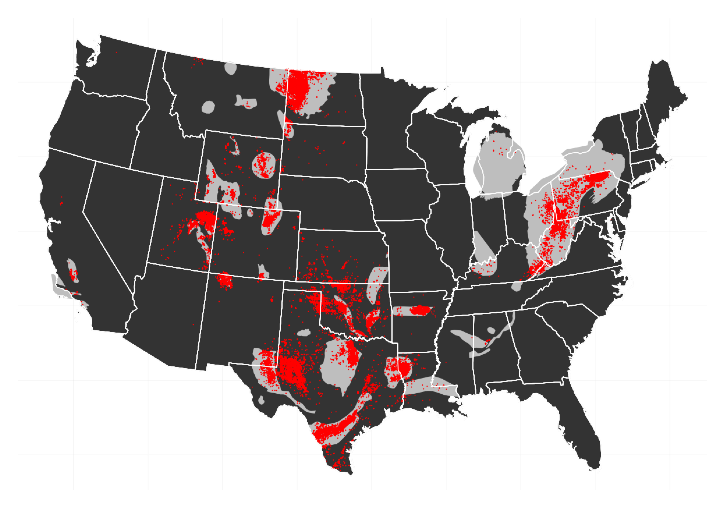
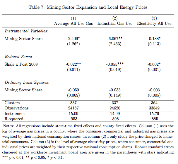
In my paper on the impact of the shale oil and gas boom in the US, I run various instrumental variables specifications. For these, it is nice to stack the regression results one on the other – in particular, to have one row for the IV results, one row for the Reduced Form and maybe one row for plain OLS to see how the IV may turn coefficients around.
I found that as of now – there is no way to do that directly; please correct me if I am wrong.
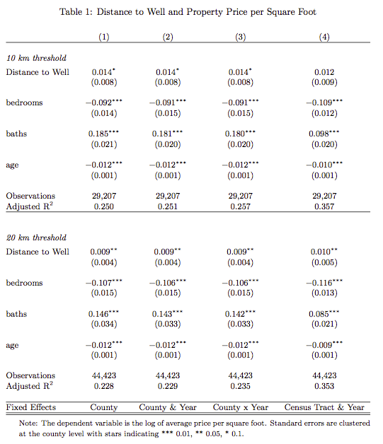
The layout I have in mind is as in the screenshot of my table.
 Â In Stata, this can be accomplished through the use of esttab with the fragment, and append feature. This appends successive rows to an existing table and you can label the rows using the “refcat” option.
 In Stata, this can be accomplished through the use of esttab with the fragment, and append feature. This appends successive rows to an existing table and you can label the rows using the “refcat” option.
However, in R this is not possible as of yet. I have mainly worked with stargazer, as Marek has added felm objects for high dimensional fixed effects to be handled by his stargazer package.
The following functions are a “hack” that extracts the particular rows from the generated latex code by the stargazer package.
You can then piece the table together by combining the individual elements. The idea is that you have a single stargazer command that is passed to the various functions that extract the different features. Obviuously, this can be done a lot more elegant as the code is extremely hacky, but it does work
Marek has said that he is thinking of incorporating a stacking option into stargazer, but for now, my hack works reasonably well. The key thing to realise is that stargazer calls have the option to return
The following character strings can be used in the table.layout and omit.table.layout arguments of the stargazer command.
“-“ single horizontal line “=” double horizontal line “-!” mandatory single horizontal line “=!” mandatory double horizontal line “l” dependent variable caption “d” dependent variable labels “m” model label “c” column labels “#” model numbers “b” object names “t” coefficient table “o” omitted coefficient indicators “a” additional lines “n” notes “s” model statistics
The following functions will simply extract the rows that are being returned.
stargazer.keepcolnums<-function(call="") {
command<-gsub("\\)$",", table.layout='#'\\)",command)
call<-eval(parse(text=command))
bounds<-grep("tabular",call)
row1<- call[(bounds[1]+1):(bounds[2]-1)]
row1<-gsub("^\\\\\\\\\\[-1\\.8ex\\]\\\\hline $", "", row1)
row1<-gsub("^\\\\hline \\\\\\\\\\[-1\\.8ex\\] $","",row1)
row1<-row1[row1!=""]
}
stargazer.keeprow<-function(call="") {
command<-gsub("\\)$",", table.layout='t'\\)",command)
call<-eval(parse(text=command))
bounds<-grep("tabular",call)
row1<- call[(bounds[1]+1):(bounds[2]-1)]
row1<-gsub("^\\\\\\\\\\[-1\\.8ex\\]\\\\hline $", "", row1)
row1<-gsub("^\\\\hline \\\\\\\\\\[-1\\.8ex\\] $","",row1)
row1<-row1[row1!=""]
}

stargazer.keepstats<-function(call="") {
command<-gsub("\\)$",", table.layout='s'\\)",command)
call<-eval(parse(text=command))
row1<-gsub("(.*)\\\\\\\\\\[-1\\.8ex\\](.*)(\\\\end\\{tabular\\})(.*)","\\2",paste(call,collapse=" "))
row1
}
stargazer.begintable<-function(call="") {
command<-gsub("\\)$",", table.layout='m'\\)",command)
call<-eval(parse(text=command))
row1<-paste("\\begin{tabular}",gsub("(.*)\\\\begin\\{tabular\\}(.*)(\\\\end\\{tabular\\})(.*)","\\2",paste(call,collapse="\n")),sep="")
row1
}
stargazer.varlabels<-function(call="") {
command<-gsub("\\)$",", table.layout='d'\\)",command)
call<-eval(parse(text=command))
row1<-paste("\\begin{tabular}",gsub("(.*)\\\\begin\\{tabular\\}(.*)(\\\\end\\{tabular\\})(.*)","\\2",paste(call,collapse="\n")),sep="")
row1
}

stargazer.keepcollabels<-function(call="") {
command<-gsub("\\)$",", table.layout='c'\\)",command)
call<-eval(parse(text=command))
row1<-gsub("(.*)\\\\\\\\\\[-1\\.8ex\\](.*)(\\\\end\\{tabular\\})(.*)","\\2",paste(call,collapse=" "))
row1
}

stargazer.keepomit<-function(call="") {
command<-gsub("\\)$",", table.layout='o'\\)",command)
call<-eval(parse(text=command))
row1<-gsub("(.*)\\\\\\\\\\[-1\\.8ex\\](.*)(\\\\end\\{tabular\\})(.*)","\\2",paste(call,collapse="\n"))
row1
}
It easiest to see how you can use these functions to construct stacked regression output by giving a simple example.
###the global command to be passed to the hacky ###functions that extract the individual bits
## OLS is a list of OLS results from running the
## lfe command
command<-'stargazer(OLS , keep=c("post08shale:directutilityshare","post08shale"), covariate.labels=c("Energy Intensity x Shale","Shale"), header=FALSE, out.header=FALSE, keep.stat=c("n","adj.rsq"))'

begintable<-stargazer.begintable(command)
###some multicolumn to combine
collcombine<-c("& \\multicolumn{4}{c}{Tradable Goods Sector Only} & \\multicolumn{3}{c}{Additional Sectors} & \\cmidrule(lr){2-5} \\cmidrule(lr){6-8}")
collabel<-stargazer.keepcollabels(command)
colnums<-stargazer.keepcolnums(command)
##plain OLS row
row1<-stargazer.keeprow(command)
##the stats part for the OLS (number of Obs, R2)
stats<-stargazer.keepstats(command)
##the rows for the Fixed effect indicators
omitted<-stargazer.keepomit(command)

##the IV command passing a list of IV results in ## IV object
command<-'stargazer(IV , keep=c("post08anywell:directutilityshare","post08anywell"), covariate.labels=c("Energy Intensity x Anywell","Anywell"), header=FALSE, out.header=FALSE, keep.stat=c("n","adj.rsq"))'

##IV row
row2<-stargazer.keeprow(command)
footer<-c("\\end{tabular}\n" )

###now combine all the items
cat(begintable,collcombine,collabel,colnums,"\\hline \\\\\\emph{Reduced Form} \\\\",row1,""\\hline \\\\\\emph{Reduced Form} \\\\",row2,stats,"\\hline\\hline",footer, file="Draft/tables/energyintensity.tex", sep="\n")
I know the solution is a bit hacky, but it works and does the trick.