Category Archives: Programming

Correction For Spatial And Temporal Auto-Correlation In Panel Data: Using R To Estimate Spatial HAC Errors Per Conley

Darin Christensen and Thiemo Fetzer


tl;dr: Fast computation of standard errors that allows for serial and spatial auto-correlation.


Economists and political scientists often employ panel data that track units (e.g., firms or villages) over time. When estimating regression models using such data, we often need to be concerned about two forms of auto-correlation: serial (within units over time) and spatial (across nearby units). As Cameron and Miller (2013) note in their excellent guide to cluster-robust inference, failure to account for such dependence can lead to incorrect conclusions: “[f]ailure to control for within-cluster error correlation can lead to very misleadingly small standard errors…” (p. 4).

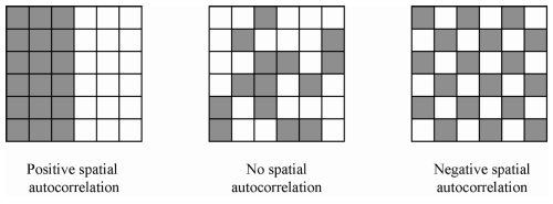
Conley (1999, 2008) develops one commonly employed solution. His approach allows for serial correlation over all (or a specified number of) time periods, as well as spatial correlation among units that fall within a certain distance of each other. For example, we can account for correlated disturbances within a particular village over time, as well as between that village and every other village within one hundred kilometers. As with serial correlation, spatial correlation can be positive or negative. It can be made visually obvious by plotting, for example, residuals after removing location fixed effects.

Example Visualization of Spatial Correlation
Example Visualization of Spatial Correlation from Radil, S. Matthew, Spatializing Social Networks: Making Space for Theory In Spatial Analysis, 2011.

We provide a new function that allows R users to more easily estimate these corrected standard errors. (Solomon Hsiang (2010) provides code for STATA, which we used to test our estimates and benchmark speed.) Moreover using the excellent lfe, Rcpp, and RcppArmadillo packages (and Tony Fischetti’s Haversine distance function), our function is roughly 20 times faster than the STATA equivalent and can scale to handle panels with more units. (We have used it on panel data with over 100,000 units observed over 6 years.)

This demonstration employs data from Fetzer (2014), who uses a panel of U.S. counties from 1999-2012. The data and code can be downloaded here.


STATA Code:

We first use Hsiang’s STATA code to compute the corrected standard errors (spatHAC in the output below). This routine takes just over 25 seconds.

cd "~/Dropbox/ConleySEs/Data"
clear; use "new_testspatial.dta"

tab year, gen(yy_)
tab FIPS, gen(FIPS_)

timer on 1
ols_spatial_HAC EmpClean00 HDD yy_*FIPS_2-FIPS_362, lat(lat ) lon(lon ) t(year) p(FIPS) dist(500) lag(5) bartlett disp

# *-----------------------------------------------
# *    Variable |   OLS      spatial    spatHAC
# *-------------+---------------------------------
# *         HDD |   -0.669     -0.669     -0.669
# *             |    0.608      0.786      0.838

timer off 1
timer list 1
#  1:     24.8 /        3 =      8.2650

R Code:

Using the same data and options as the STATA code, we then estimate the adjusted standard errors using our new R function. This requires us to first estimate our regression model using the felm function from the lfe package.

# Loading sample data:
dta_file <- "~/Dropbox/ConleySEs/Data/new_testspatial.dta"
DTA <-data.table(read.dta(dta_file))
setnames(DTA, c("latitude", "longitude"), c("lat", "lon"))

# Loading R function to compute Conley SEs:
source("~/Dropbox/ConleySEs/ConleySEs_17June2015.R")

ptm <-proc.time()

# We use the felm() from the lfe package to estimate model with year and county fixed effects.
# Two important points:
# (1) We specify our latitude and longitude coordinates as the cluster variables, so that they are included in the output (m).
# (2) We specify keepCx = TRUE, so that the centered data is included in the output (m).

m <-felm(EmpClean00 ~HDD -1 |year +FIPS |0 |lat +lon,
  data = DTA[!is.na(EmpClean00)], keepCX = TRUE)

coefficients(m) %>%round(3) # Same as the STATA result.
   HDD 
-0.669 

We then feed this model to our function, as well as the cross-sectional unit (county FIPS codes), time unit (year), geo-coordinates (lat and lon), the cutoff for serial correlation (5 years), the cutoff for spatial correlation (500 km), and the number of cores to use.

SE <-ConleySEs(reg = m,
    unit = "FIPS", 
    time = "year",
    lat = "lat", lon = "lon",
    dist_fn = "SH", dist_cutoff = 500, 
    lag_cutoff = 5,
    cores = 1, 
    verbose = FALSE) 

sapply(SE, sqrt) %>%round(3) # Same as the STATA results.
        OLS     Spatial Spatial_HAC 
      0.608       0.786       0.837 
proc.time() -ptm
   user  system elapsed 
  1.619   0.055   1.844 

Estimating the model and computing the standard errors requires just over 1 second, making it over 20 times faster than the comparable STATA routine.


R Using Multiple Cores:

Even with a single core, we realize significant speed improvements. However, the gains are even more dramatic when we employ multiple cores. Using 4 cores, we can cut the estimation of the standard errors down to around 0.4 seconds. (These replications employ the Haversine distance formula, which is more time-consuming to compute.)

pkgs <-c("rbenchmark", "lineprof")
invisible(sapply(pkgs, require, character.only = TRUE))

bmark <-benchmark(replications = 25,
  columns = c('replications','elapsed','relative'),
  ConleySEs(reg = m,
    unit = "FIPS", time = "year", lat = "lat", lon = "lon",
    dist_fn = "Haversine", lag_cutoff = 5, cores = 1, verbose = FALSE),
  ConleySEs(reg = m,
    unit = "FIPS", time = "year", lat = "lat", lon = "lon",
    dist_fn = "Haversine", lag_cutoff = 5, cores = 2, verbose = FALSE),
  ConleySEs(reg = m,
    unit = "FIPS", time = "year", lat = "lat", lon = "lon",
    dist_fn = "Haversine", lag_cutoff = 5, cores = 4, verbose = FALSE))
bmark %>%mutate(avg_eplased = elapsed /replications, cores = c(1, 2, 4))
  replications elapsed relative avg_eplased cores
1           25   23.48    2.095      0.9390     1
2           25   15.62    1.394      0.6249     2
3           25   11.21    1.000      0.4483     4

Given the prevalence of panel data that exhibits both serial and spatial dependence, we hope this function will be a useful tool for applied econometricians working in R.


Feedback Appreciated: Memory vs. Speed Tradeoff

This was Darin’s first foray into C++, so we welcome feedback on how to improve the code. In particular, we would appreciate thoughts on how to overcome a memory vs. speed tradeoff we encountered. (You can email Darin at darinc[at]stanford.edu.)

The most computationally intensive chunk of our code computes the distance from each unit to every other unit. To cut down on the number of distance calculations, we can fill the upper triangle of the distance matrix and then copy it to the lower triangle. With [math]N[/math] units, this requires only  [math](N (N-1) /2)[/math] distance calculations.

However, as the number of units grows, this distance matrix becomes too large to store in memory, especially when executing the code in parallel. (We tried to use a sparse matrix, but this was extremely slow to fill.) To overcome this memory issue, we can avoid constructing a distance matrix altogether. Instead, for each unit, we compute the vector of distances from that unit to every other unit. We then only need to store that vector in memory. While that cuts down on memory use, it requires us to make twice as many   [math](N (N-1))[/math]  distance calculations.

As the number of units grows, we are forced to perform more duplicate distance calculations to avoid memory constraints – an unfortunate tradeoff. (See the functions XeeXhC and XeeXhC_Lg in ConleySE.cpp.)


sessionInfo()
R version 3.2.2 (2015-08-14)
Platform: x86_64-apple-darwin13.4.0 (64-bit)
Running under: OS X 10.10.4 (Yosemite)

locale:
[1] en_GB.UTF-8/en_GB.UTF-8/en_GB.UTF-8/C/en_GB.UTF-8/en_GB.UTF-8

attached base packages:
[1] stats     graphics  grDevices utils     datasets  methods  
[7] base     

other attached packages:
 [1] RcppArmadillo_0.5.400.2.0 Rcpp_0.12.0              
 [3] geosphere_1.4-3           sp_1.1-1                 
 [5] lfe_2.3-1709              Matrix_1.2-2             
 [7] ggplot2_1.0.1             foreign_0.8-65           
 [9] data.table_1.9.4          dplyr_0.4.2              
[11] knitr_1.11               

loaded via a namespace (and not attached):
 [1] Formula_1.2-1    magrittr_1.5     MASS_7.3-43     
 [4] munsell_0.4.2    xtable_1.7-4     lattice_0.20-33 
 [7] colorspace_1.2-6 R6_2.1.1         stringr_1.0.0   
[10] plyr_1.8.3       tools_3.2.2      parallel_3.2.2  
[13] grid_3.2.2       gtable_0.1.2     DBI_0.3.1       
[16] htmltools_0.2.6  yaml_2.1.13      assertthat_0.1  
[19] digest_0.6.8     reshape2_1.4.1   formatR_1.2     
[22] evaluate_0.7.2   rmarkdown_0.8    stringi_0.5-5   
[25] compiler_3.2.2   scales_0.2.5     chron_2.3-47    
[28] proto_0.3-10    

Leveraging R for Econ Job Market


[UPDATE] I just was told that the new features on EJM actually allow you to download an XLS spreadsheet of the job listings on EJM. This is accessible when you login to myeconjobmarket.org and is part of their new AIMS (Application and Interview Management System).

I wanted to describe a little helper I am using to help refine the places I want to apply at since I am going to be on the Economics Job Market this year.

The two main websites were job openings are advertised are:

Now JOE has a really nice feature where you can download simply all job openings into a nice spreadsheet. This allows you to browse through and refine your search. Econ Job Market does not have such a feature.

The Listing page is quite annoying…

ejm-listing


If you want more details for a job opening, such as a description of the fields and application requirements, you will have to click on “more info…”. In the JOE spreadsheet, you have all that information at once.

I wanted to create a JOE like spreadsheet using the openings from EJM. Some of which, of course, do overlap. But for some reason, some jobs are only on EJM but not on JOE.

So how can we use R to help us do that?

The first thing I wanted to do is get the simple listings on the main application page from EJM as a spreadsheet. You can simply download the main listings file and extract the pieces of information. Most important is the “posid” field, which is the position ID contained in the EJM URL. This will give you a direct link to the HTML page of the job opening and it also tells you whether you can apply through EJM.

This leaves you with a listing of EJM links to jobs, their position ID and the EJM Application Link in case the Job Opening accepts applications through EJM. Now you can proceed to simply download all the HTML files using a batch downloader such as DownThemAll. If you want to do that, you can print out a list:

cat(EJM$url, sep="\n")

and enter them into Down Them All. Alternatively you can iterate through the list of links and send HTTP queries to get the details from each job separately. This is part of the next lines of code:

This renders us with a nice csv that we can browse quickly through in Excel…for convenience you can download the listings as of 23-10-2014 below. Good luck for your applications!

econjobmarket-23-10-2014

Is rainfall reporting endogenous to conflict?

For my paper on the impact of social insurance on the dynamics of conflict in India, I use some new remote sensed weather data. The data comes from the Tropical Rainfall Measuring Mission (TRMM) satellites. The satellite carries a set of five instruments, and is essentially a rainfall radar located in outer space.

As a robustness check I needed to verify that my main results go through using other rainfall data. In the paper I try to make a humble case in favour of using remote sensed data where possible. The key reason being that the  TRMM data comes from the same set of instruments over time, rather than from input sources that could be varying with e.g., economic conditions. This is a problem that has been identified by climatologist, who try to correct for systematic biases that could arise from the fact that weather stations are more likely to be located in places with a lot of economic activity.

At first I was a bit reluctant as it is quite heavy data that needs to be processed. Nevertheless, thorough analysis required me to jump the hoop and obtain secondary rainfall data sources. I chose the GPCC monthly rainfall data for verification of my results, since these have been used by many other authors in the past in similar contexts. The data is based on rain gauge measurements and is available for the past 100 years.

The raw data is quite heavy ; the monthly rainfall rate data  for the whole world at at 0.5 degree resolution would amount to about 150 million rows of data for the period from 1961-2010. If you drop the non-land grid cells, this reduces the size dramatically to only 40 million rows. Below is a bit of code that   loads in the data once you have downloaded the ASCII source files from the GPCC website. On my personal website, I make a dta and an rdata file available for the whole world. There are three variables appearing in that order: (1) the rainfall rate, (2) the rainfall normals and (3) an integer that gives the number of reporting rain gauges that fall in a grid cell in a particular month.

It turns out that all my results are robust to using this data. However, I do find something that is quite neat. It turns out that, if a district experienced some insurgency related conflict in the previous year,  it is less likely that this district has an active rain gauge reporting data in subsequent years. While it is a no-brainer that places with severe conflict do not have functioning weather reporting, these results suggest  that reporting may also be systematically affected in places with relatively low intensity of conflict – as is the case of India.

While I do not want to overstate the importance of this, it provides another justification of why it makes sense for economists to be using  remotely sensed weather data. This is not to say that ground based data is not useful. Quite the reverse, ground based data is more accurate in many ways, which makes it very important for climatologist. As economist, we are worried about systematic measurement error that correlates with the economic variables we are studying. This is were remote sensed data provides advantages as it does not “decide” to become less accurate in places that are e.g. less developed, suffer from conflict or simply, have nobody living there.

Here the function to read in the data and match to district centroids, you need some packages.

#########LOAD GPPC NOTE THAT YOU NEED TO SUBSET 
THE DATA IF YOU DONT WANT TO END UP WITH A HUGE 
DATA OBJECT

loadGPCC<-function(ff, COORDS) {
yr<-as.numeric(gsub("(.*)\\_([0-9]{2})([0-9]{4})","\\3",ff))
month<-as.numeric(gsub("(.*)\\_([0-9]{2})([0-9]{4})","\\2",ff))
temp<-data.table(data.frame(cbind(COORDS,
read.table(file=paste("Rainfall/gpcc_full_data_archive_v006_05_degree_2001_2010/",
ff,sep=""), header=FALSE, skip=14))))

###YOU COULD SUBSET THE DATA BY EXTENT HERE IF 
YOU DONT WANT TO GET IT FOR THE WHOLE WORLD
##E.G. SUBSET FOR BY BOUNDING BOX
##temp<-temp[x>=73 & x<=136 & y>=16 & y<=54]

temp<-cbind("year"= yr, "month"=month, temp)
gc("free")
temp
}

################
#####
ffs<-list.files("Rainfall/
gpcc_full_data_archive_v006_05_degree_2001_2010")

###THIS DEFINES THE GRID STRUCTURE OF THE DATA
###YOU MAY NEED TO ADJUST IF YOU WORK WITH A 
COARSER GRID
xs=seq(-179.75,179.75,.5)
ys=seq(89.75,-89.75,-.5)
COORDS<-do.call("rbind", lapply(ys, function(x) cbind("x"=xs,"y"=x)))

system.time(GPCC<-do.call("rbind", lapply(1:length(ffs), function(x) loadGPCC(ffs[x], COORDS))))

###MATCHING THIS TO SHAPEFILE?
##YOU COULD MATCH CENTROIDS OF DISTRICTS TO THE 
NEAREST GRID CELL - THE FOLLOWING FUNCTION WOULD 
DO THAT

###find nearest lat / lon pair
##you may want to vectorise this
NEAREST<-NULL
for(k in 1:nrow(CENTROIDS)) {
cat(k," ")
temp<-distHaversine(CENTROIDS[k,c("x","y"),with=F], 
GPCC.coords[, c("delx","dely"), with=F])
NEAREST<-rbind(NEAREST, cbind(CENTROIDS[k],GPCC.coords[which(temp==
min(temp))]))

}


Deploying Shiny Server on Amazon: Some Troubleshoots and Solutions

I really enjoyed Treb Allen‘s tutorial on deploying a Shiny server on an Amazon Cloud Instance. I used this approach for my shiny app that is a map highlighting the economic impact of the recent shale oil and gas boom on the places where the actual extraction happens. The easiest way to proceed is to use the AMI Image, which basically is like a virtual box image just running on Amazon Cloud. It has the basic Shiny-server up and running. Along the way, I came across a few troubleshoots for which there are simple solutions.

I cant seem to access the Shiny server through the Browser?

Right after the installation and setting up of the Amazon Instance, I tried to access the shiny server using the public DNS, in my case that was

Public DNS: ec2-54-84-227-28.compute-1.amazonaws.com

However, this did not work since the shiny-server is listening on port 3838 and you need to allow incoming traffic on that port. The way to manage that in the EC2 Dashboard is to go change the security group that is assigned to the instance that you are running. You need to add a rule to allow incoming traffic on port 3838.

Once this is done, you should be able to go to your public DNS, in my case the request URL in the browser now is:

ec2-54-72-74-90.eu-west-1.compute.amazonaws.com:3838/shale-economic-impact/ in your browser

Where are the shiny-apps located?

The standard shiny apps that are preinstalled are  located in
“/var/shiny-server/www” If you ssh into your EC2 instance, you can go to that folder.

I installed packages, but my shiny application can not load them?

The problem is most likely that you are logged in as ec2-user, where you have your own dedicated library path. In order to install R packages system wide, you need to change to root by doing:

sudo -i
##install now your R packages,
R CMD INSTALL ...
exit

The exit part is important as then you turn off administrator rights.

When I run the app, I get Javascript Error  “The application unexpectedly exited. Diagnostic information has been dumped to the JavaScript error console.”?

It could be that your EC2 instance is not powerful enough. I had that problem because the dataset that was loaded was too big, which creates a time-out. One way to overcome this is to start a medium instance rather than a micro instance. Please be aware that this is not part of the free usage tier and you will be billed for usage. However, an alternative simple  fix by editing the config file. It could be that you are hitting a time-out.

In the shiny-server configuration help, there are two timeouts that can be set in the free shiny server version.

app_init_timeout — Describes the amount of time (in seconds) to wait for an application to start. After this many seconds if the R process still has not become responsive, it will be deemed an unsuccessful startup and the connection will be closed.

app_idle_timeout — Defines the amount of time (in seconds) an R process with no active connections should remain open. After the last connection disconnects from an R process, this timer will start and, after the specified number of seconds, if no new connections have been created, the R process will be killed.

It could be that the javascript error is thrown, because the R process was killed.  You can edit the configuration file to increase the time-out periods, adding:

# Instruct Shiny Server to run applications as the user "shiny"

run_as shiny;

# Define a server that listens on port 3838

server {

listen 3838;

# Define a location at the base URL

location / {

# Host the directory of Shiny Apps stored in this directory
site_dir /var/shiny-server/www;
# Log all Shiny output to files in this directory
log_dir /var/log/shiny-server;
# When a user visits the base URL rather than a particular application,
# an index of the applications available in this directory will be shown.

directory_index off;
app_init_timeout 250;

}

}

This brings us right to the next question,…

Where do I find my shiny server configuration file?

There is a hard coded configuration file, but in the search path there is one located in:

/etc/shiny-server/shiny-server.conf

here you can do the above edits. After you have  done the edits you want to reload the configuration…

How do I reload the Configuration File, how to start or stop the shiny server?

#reload without restarting
sudo reload shiny-server
#stop the shiny server 
sudo stop shiny-server
#start it...
sudo stop shiny-server

Copying files from your local machine to the AWS Instance?

You can use “scp” for secure copying, e.g.

To download files from your instance:
scp -i frackingshiny-eu-west-1.pem ec2-user@ec2-54-72-74-90.eu-west-1.compute.amazonaws.com:/var/shiny-server/www/shale-economic-impact.zip

To upload files to your instance:
scp -r -i frackingshiny-eu-west-1.pem “/Users/thiemo/shale-economic-impact.zip” ec2-user@ec2-54-72-74-90.eu-west-1.compute.amazonaws.com:/var/shiny-server/www/

I plan to add more troubleshoots – if you have come across some error for which you had to find a solution, feel free to comment and I ll amend the list.

Regressions with Multiple Fixed Effects – Comparing Stata and R

In my paper on the impact of the recent fracking boom on local economic outcomes, I am estimating models with multiple fixed effects. These fixed effects are useful, because they take out, e.g. industry specific heterogeneity at the county level – or state specific time shocks.

The models can take the form:

[math]y_{cist} = \alpha_{ci} + b_{st} + \gamma_{it}+ X_{cist}'\beta + \epsilon_{cist}[/math]  

where [math]\alpha_{ci}[/math] is a set of county-industry, [math]b_{ci}[/math] a set of state-time and [math]\gamma_{it}[/math] is a set of industry-time fixed effects.

Such a specification takes out arbitrary state-specific time shocks and industry specific time shocks, which are particularly important in my research context as the recession hit tradable industries more than non-tradable sectors, as is suggested in Mian, A., & Sufi, A. (2011). What Explains High Unemployment ? The Aggregate Demand Channel.

How can we estimate such a specification?
Running such a regression in R with the lm or reg in stata will not make you happy, as you will need to invert a huge matrix. An alternative in Stata is to absorb one of the fixed-effects by using xtreg or areg. However, this still leaves you with a huge matrix to invert, as the time-fixed effects are huge; inverting this matrix will still take ages.

However, there is a way around this by applying the Frisch-Waugh Lovell theorem iteratively (remember your Econometrics course?); this basically means you iteratively take out each of the fixed effects in turn by demeaning the data by that fixed effect. The iterative procedure is described in detail in Gaure (2013), but also appears in Guimaraes and Portugal(2010).

Simen Gaure has developed an R-package called lfe, which performs the demeaning for you and also provides the possibility to run instrumental variables regressions; it theoretically supports any dimensionality of fixed effects. The key benefit of Simen Gaure’s implementation is the flexibility, the use of C in the background for some of the computing and its support for multicore processing, which speeds up the demeaning process dramatically, especially the larger your samples get..

In Stata there is a package called reg2hdfe and reg3hdfe which has been developed by Guimaraes and Portugal (2010). As the name indicates, these support only fixed effects up to two or three dimensions.

Lets see how – on the same dataset – the runtimes of reg2hdfe and lfe compare.

Comparing Performance of Stata and R

I am estimating the following specification

[math]y_{cist} = \alpha_{ci} + b_{sit} + \gamma_{it}+ X_{cist}'\beta + \epsilon_{cist}[/math]  

where [math]\alpha_{ci}[/math] is a set of county-industry, [math]b_{ci}[/math] a set of state-time fixed effects. There are about 3000 counties in the dataset and 22 industries. Furthermore, there are 50 states and the time period is also about 50 quarters. This means – in total – there are 3000 x 22 = 66,000 county-industry fixed effects to be estimated and 22 x 50 x 50 = 55,000 time fixed effects to be estimated. The sample I work with has sufficient degrees of freedom to allow the estimation of such a specification – I work with roughly 3.7 million observations.

I have about 10 covariates that are in [math]X_{cist}[/math], i.e. these are control variables that vary within county x industry over state x industry x time.

Performance in Stata

In order to time the length of a stata run, you need to run
set rmsg on, which turns on a timer for each command that is run.

The command I run in stata is

reg2hdfe logy x1-x10,  id1(sitq ) id2(id) cluster(STATE_FIPS )

You should go get a coffee, because this run is going to take quite a bit of time. In my case, it took t=1575.31, or just about 26 minutes.

Performance in R 
In order to make the runs of reg2hdfe and lfe, we need to set the tolerance level of the convergence criterion to be the same in both. The standard tolerance in Stata is set at $$1e^{-6}$$, while for lfe package it is set at $$1e^{-8}$$. In order to make the runs comparable you can set the options in the R package lfe options explicitly:

options(lfe.eps=1e-6)

The second change we need to make is to disallow lfe to use multiple cores, since reg2hdfe uses only a single thread. We can do this by setting:

options(lfe.threads=1)

Now lets run this in R using:

system.time(summary(felm(log(y) ~ x1 + x2 +x3 +x4 + x5 + x6 + x7 +x8 + x9 + x10 + G(id)+G(sitq),
data=EMP, cluster=c("STATE_FIPS"))))

The procedure converges in a lot quicker than Stata…

 user system elapsed 
208.450 23.817 236.831 

It took a mere 4 minutes. Now suppose I run this in four separate threads…

user system elapsed 
380.964 23.540 177.520


Running this on four threads saves about one minute in processing time; not bad, but not too much gained; the gains from multi-threading increase, the more fixed-effects are added and the larger the samples are.

Classi-Compare of Raster Satellite Images – Before and After

For my research on the effect of power outages on fertility , we study a period of extensive power rationing that lasted for almost a whole year and affected most of Latin America, but in particular, it affected Colombia. The key difficult was to determine which areas were exposed to the power-outage and the extent to which this was the case. This is not straightforward, since there does not exist household- or even municipality level consumption data.

But here is how R and Satellite Data can help. In particular, we study the night light series obtained from the Defense Meterological Sattelite Program, which has been discussed by Jeffrey before.

We simply look for abnormal variation in municipality level light-emitting intensity from 1992 to 1993.

Here is some code that generates some Raster-Maps using the package rasterVis , and uses jQuery to generate a fancy before and after comparison to highlight the year-on-year changes in light intensity of 1992 compared to 1993.

###load the raster images
tif<-"F101992.v4b_web.stable_lights.avg_vis.tif"
f151 = raster(tif)

tif<-"F101993.v4b_web.stable_lights.avg_vis.tif"
f152 = raster(tif)

##crop a smaller window to plot

e = extent(-78,-72,2,8)
#e = extent(-80,-78,-4.6,-2)
rn= crop(f151, e)
rn2= crop(f152, e)

### do a logarithmic transformation to highlight places that receive not much, but some light.

rn<-log(rn+1)
png("1992.png")
p <- levelplot(rn, layers=1, margin=FALSE,col.regions = gray(0:100/100))
p + layer(sp.polygons(COLPOB, lwd=.25, linetype=2, col='darkgray'))
dev.off()

rn2<-log(rn2+1)
png("1993.png")
p <- levelplot(rn2, layers=1, margin=FALSE,col.regions = gray(0:100/100))
p + layer(sp.polygons(COLPOB, lwd=.25, linetype=2, col='darkgray'))
dev.off()

Now with this together, you can create a fancy slider as I have seen on KFOR — comparing satellite pictures of towns before and after a tornado went through them.

The code is essentially just borrowed from that TV station and it loads the javascript from their server; it is essentially just a clever use of jQuery and is maybe something that could or is already implemented in an R reporting package? Do you know of such a function?

Anyways, all you need is a slider.html page that contains the code referring to the two picture sources; the code is simple:


<!DOCTYPE html>
<html>
  <head>
    <meta http-equiv="Content-Type" content="text/html; charset=UTF-8">
    <script src="https://ajax.googleapis.com/ajax/libs/jquery/1.8.3/jquery.min.js"></script>
    <script src="http://cache.ltvcms.com/localtv/tornado2/js/jquery.classycompare.js"></script>
    <link rel="stylesheet" type="text/css" href="http://cache.ltvcms.com/localtv/tornado2/css/jquery.classycompare.css">
    <style type="text/css">.sample1 {width:725px; height:725px;}.sample2 {width:725px; height:725px;}.sample3 {width:725px; height:725px;}</style>
  </head>
  <body>
    <div id="wrapper">
      <div class="container_6 clearfix">
        <section class="main-section grid_6">
          <div class="main-content">
            <section class="clearfix">
              <div>
                <div class="container" style="position:relative">
                  <div class="sample1"> <img src="1992municio.png"
                      alt="Before"
                      height="725px"
                      width="725px">
                    <img src="1993municio.png"
                      alt="After"
                      height="725px"
                      width="725px">
                  </div>
                </div>
                <script>
                                        $(window).load(function() {
                                            $('.sample1').ClassyCompare({
                                                defaultgap:50,
                                                leftgap:0,
                                                rightgap:10,
                                                caption: true,
                                                reveal: 0.5
                                            });
                                        });
                                    </script> </div>
            </section>
          </div>
        </section>
      </div>
    </div>

  </body>
</html>


This is how it looks — I know the stuff is not perfectly aligned, partly because when cropping the picture I made a mistake and could not be bothered with fixing it.

Have fun!


Computing Maritime Routes in R

Thanks to the attention my paper on the cost of Somali piracy has received, a lot of people have approached me to ask how I computed the maritime routes. It is not a very difficult task using R. The key ingredient is a map of the world, that can be rasterized into a grid; all the landmass needs to be assigned an infinite cost of crossing and last but not least — one needs to compute the actual routes.

What packages do I need?

library(gdistance)
library(maptools)
data(wrld_simpl)
library(data.table)

The package gdistance does most of the actual work of computing the routes. The wrld_simpl map provides what is needed to generate a raster.

Generating a Raster

#create a raster from shape files
shp <- wrld_simpl
r <- raster()
r <-rasterize(shp, r, progress='text')

After the raster is generated, we can proceed by making landmass impassable for vessels.

#make all sea = -999
r[is.na(r)] <- -999
#this turns all landmass to missing
r[r>-999] <- NA
#assign unit cost to all grid cells in water
r[r==-999] <- 1

There are a few more things to do, such as opening up the Suez Canal and some other maritime passages — one needs to find the right grid cells for this task. In the next step we can transform the raster into a transition layer matrix, that comes from the gdistance package. It is a data construct that essentially tells us how one can move from one cell to the other — you can allow diagonal moves by allowing the vessel to move into all 8 adjacent grid cells. There is also a geo-correction necessary, as the diagonals are longer distances than the straight-line moves.

tr <- transition(r, mean, directions = 8)
tr <- geoCorrection(tr, "c")

Well — and thats basically it — of course, there are a few bits and pieces that need additional work — like adding heterogenuous costs as one can imagine exist due to maritime currents and so on. Furthermore, there is a whole logic surrounding the handling of the output and the storing in a local database for further use and so on.

But not to bore you with that — how can I obtain the distance between A and B? This uses Dijkstra’s Algorithm and is called through the gdistance function “shortestPath”.

AtoB <- shortestPath(tr, as.numeric(start[1:2]), as.numeric(end[1:2]), output = "SpatialLines")

Using this output, you can then generate fancy graphs such as …


Starting Multiple Stata Instances on Mac

I found it useful to have multiple Stata instances running on my Mac, in particular, if I use one instance to clean the data before running merge commands. It is always annoying if the merging does not work out or throws an error and then, one would have to clear the current instance and open the DTA file that was messing up the merge.

Its a simple command that allows you to open multiple Stata instances on a Mac:

open -n /Applications/Stata12_OSX/StataSE.app

You can also define an alias command in your .bash_profile,

alias stata='open -n /Applications/Stata12_OSX/StataSE.app'
Good luck!


R function: generate a panel data.table or data.frame to fill with data

I have started to work with R and STATA together. I like running regressions in STATA, but I do graphs and setting up the dataset in R. R clearly has a strong comparative advantage here compared to STATA. I was writing a function that will give me a (balanced) panel-structure in R. It then simply works by joining in the additional data.tables or data.frames that you want to join into it.

It consists of two functions:

timeVector <- function(starttime,endtime,timestep="months") {

starttime<- as.POSIXct(strptime(starttime, '%Y-%m-%d'))
endtime<- as.POSIXct(strptime(endtime, '%Y-%m-%d'))
if(timestep=="quarters") {
timestep="months"
ret<-seq(from=as.POSIXct(starttime), to=as.POSIXct(endtime), by=timestep)
quarter <- gsub("(^[123]{1}$)", 1, month(ret))
quarter <- gsub("(^[456]{1}$)", 2, quarter)
quarter <- gsub("(^[789]{1}$)", 3, quarter)
quarter <- as.numeric(gsub("(^[102]{2}$)", 4, quarter))

ret<-paste(year(ret),quarter,sep="-")
ret<-unique(ret)
} else {

ret<-seq(from=as.POSIXct(starttime), to=as.POSIXct(endtime), by=timestep)
}
ret

}

This first function generates the time-vector, you need to tell it what time-steps you want it to have.

panelStructure <- function(group,timevec) {
tt<-rep(timevec,length(group))
tt2 <- as.character(sort(rep(group,length(timevec))))
mat <- cbind("group"=data.frame(tt2),"timevec"=data.frame(tt))
names(mat)<-c("group","timevec")
mat
}

This second function then generates the panel-structure. You need to give it a group vector, such as for example a vector of district names and you need  to pass it the time vector that the other function created.

Hope this is helpful to some of you.


Removing Multibyte Characters from Strings

I was a bit annoyed by the error when loading a dataset that contains multi-byte characters. R basically just chokes on them. I have not really understood the intricacies of this, but it was basically just an annoyance and since I did not really use these characters in the strings containing them, I just wanted to remove them.

The easiest solution was to use Vim with the following search and replace:

s/[\x80-\xFF]//g

Downloading All Your Pictures From iPad or iPhone

I really disklike iTunes, it is the worst piece of software I have ever come accross.  I would say that Windows has been getting better and better. I had the following problem: I uploaded quite a few pictures via iTunes onto my iPad, just because its nice to look at pictures on that machine. However, the machine with which I did the syncing broke and needed repair and somehow, I forgot to save these pictures onto a  hard drive for backup. So the only place where these pictures now rest is on my iPad.

iTunes wont allow you to copy pictures on your iPad onto a machine (only the pictures that you atually take with the iPad). This is because, these pictures *should*  be on the machine with which you synced your iPad in the first place.

However, this was not true in my case anymore. Now you could either invest some money and purchase an app that allows you to copy your picture albums from the iPad onto a Windows machine.

There is e.g. CopyTrans Suite, which is a bit costly and in the version I tried, did not copy the full resolution of the pictures (which is a rip-off!).

So I was looking into a cheap and quick solution to get the original full resolution pictures down from my iPad.

Setting things up: installing free app “WiFi Photo”
This app basically makes your photo albums available on a local webserver. Once you start the app on the iPad, it tells you an URL to brows to on your local machine. There you can see all the pictures that are on your iPad.

Logo of the Wifi Transfer appYou could now use this app to manually download the pictures, however, it is limited to 100 pictures at once and you will not get the full resolution pictures if you do a batch download.

If you browse through the app, you will notice that the URL to the full resolution pictures has the following form:

http://192.168.1.6:15555/0/fr_564.jpg

where the “0” stands for the album ID. If you have, say 2 albums on the iPad, this would take values “0” or “1”. Images are stored as consecutive numbers in each album, so the following link would go to picture number 564 in full resolution in album 0. So we will exploit this structure to do an automated batch download.

Doing an automated batch download

First, in order for this to work you need to get a a local PHP installation up and running. If you are really lazy, you could just install XAMPP. However, you can implement the code in any other coding language, e.g. in R as well.

To download all the pictures, you need to adjust and run the following script

for($k=0;$k<=3;$k++) {

for($i=1;$i<=1000;$i++) {

//adjust this
$url = "http://192.168.1.9:15555/".$k."/fr_".$i.".jpg";

//adjust this
$fn = "C:/Dokumente und Einstellungen/Thiemo/Desktop/Kolumbien/".$k."-".$i.".jpg";

//to make sure you dont redownload a file already downloaded if you want
//to run the script several times
if(!file_exists($fn)) {
if($content = file_get_contents($url)) {
$fp = fopen($fn,"a+");
fwrite($fp, $content);
fclose($fp);
}
}
}
What this script does it iterates through the albums (the first loop), in my case I have four albums. The second loop then iterates through the pictures, I simply assume that there are at most 1000 pictures in each album. Clearly, this can be made smarter, i.e. automatically find out how many pictures in each album, but this works and thats all we need.
I would recommend running the script a few times, as sometimes it is not able to retrieve the content and then, no file is created. By adding the “file_exists” check, I make sure that no picture, that has been downloaded already, is downloaded again. So if you run the script several times, it will be quicker and quicker to also pick up the last missing pictures.
Running the script takes some time as it needs to copy down each picture, and in my case this were a rough 2000 pictures. But now, they are back in the safe haven of my local machine.

Microfinance in India: Getting a sense of the geographic distribution

I am working on a review paper on microfinance in India and use data from the MIX market. Today, I was amazed by how quick I conjured a map of India with the headquarters of the microfinance institutions that report data to the MIX market depicted on that map. Ideally, I would have more geolocation data – but this is hard to come by. But what we can clearly see is the clustering of institutions in big cities and in the south, which was hit hardest by the recent crisis.

Microfinance Institutions across India


I dont think anybody has produced such a map before. In fact, I can do this for all institutions reporting data around the world, which may be interesting to see. Also, I already tried to make the size of the dot proportional to e.g. measures of real yield or color-coding the nearest neighborhood (say the neigbhouring districts) by the average loan sizes reported. Lots of things to do. Maybe thats something for the guys at MIX Market or for David Roodman who, I think has finished his open book.

The key difficulty was actually not in plotting the map (though it took some time), but in obtaining geo-data on where the headquarters of the microfinance institutions are located. I managed to obtain this data – though its not perfect – by making calls to the Google MAP API via a PHP script., basically using the following two functions:

Continue reading Microfinance in India: Getting a sense of the geographic distribution

R Function Binding Vectors and Matrices of Variable Length, bug fixed

Now this is something very geeky, but useful. I had to bind two matrices or vectors together to become a bigger matrix. However, they need not have the same number of rows or even the same row names.

The standard cbind() functions require the vectors or matrices to be compatible. The matching is “stupid”, in the sense that it ignores any order or assumes that the elements which are to be joined into a matrix have the same row names. This, of course, need not be the case. A classical merge command would fail here, as we dont really know what to merge by and what to merge on.

Ok… I am not being clear here. Suppose you want to merge two vectors

A 2
B 4
C 3

and

G 2
B 1
C 3
E 1

now the resulting matrix should be

A  2  NA
B  4  1
C  3  3
E NA  1
G NA  2

Now the following Rfunction allows you to do this. It is important however, that you assign rownames to the objects to be merged (the A,B,C,E,G in the example), as it does matching on these.

cbindM <-
function(A, v, repl=NA) {

  dif <- setdiff(union(rownames(A),rownames(v)),intersect(rownames(A),rownames(v)))
#if names is the same, then a simple cbind will do
    if(length(dif)==0) {

      A<- cbind(A,v[match(rownames(A),rownames(v))])

        rownames(A) <- rownames(v)

    }    else if(length(dif)>0) {#sets are not equal, so either matrix is longer / shorter

#this tells us which elements in dif are part of A (and of v) respectively      
      for(i in dif)     {

        if(is.element(i,rownames(A))) {
#element is in A but not in v, so add it to v and then a        

          temp<-matrix(data =repl, nrow = 1, ncol = ncol(v), byrow = FALSE, dimnames =list(i))
            v <- rbind(v,temp)

        } else {
# element is in v but not in A, so add it to A

          temp<-matrix(data = repl, nrow = 1, ncol = ncol(A), byrow = FALSE, dimnames =list(i))
            A<-rbind(A,temp)
        }
      }


      A<-cbind(A,v[match(rownames(A),rownames(v))])

    }

  A
}

Note: 09.11.2011: I fixed a bug and added a bit more functionality. You can now tell it, with what you want the missing data to be replaced. Its standard to replace it with NA but you could change it to anything you want.