Category Archives: Econometrics

Did the weather affect the #Brexit vote?

On the evening of the polling day, some parts of London and southern England were hit by very bad weather, while other areas experienced nice weather with high temperatures and sunshine. The weather could have affected the Brexit vote by affecting Turnout or by affecting Voting Intentions.

To cut a long story short: there is, using very crude data, no evidence suggesting that the rainfall affected turnout. There is weak evidence, suggesting that the good weather in parts of the country, may have induced some voters to vote leave in the “heat of the moment”. But: overall, its unlikely that this would have changed the results.

The Brexit voters had an overall decisive lead with more than a million votes. Nevertheless, it would be interesting to see whether the “Great British Summer” contributed to the result. Further, there is quite a bit of serious economics research that document relationships, for example between rainfall and conflict, or between temperatures and aggressive behavior. But how could the weather have affected the Brexit vote?

Polling on a working day Coming from Germany, it struck me as extremely odd, why polls would take place on Thursdays – a working day. I feel that this is one of those odd English institutions or traditions created by the elites to – de-facto – limit the franchise of the working class. Naturally, it is much more difficult for the (commuting) employed  to cast their vote, as they have to do it, a) either in advance through a postal vote, b) in the morning or evening hours, which coincide with the commuting hours or, c) during the day or their lunch break. However, commuting makes it difficult as voters can register only at one polling station to cast their vote.

The opportunity cost of voting is unevenly distributed. The retired or unemployed, who turned out to be, on average more likely to vote Brexit had lower opportunity cost of voting. The uneven distribution of the opportunity cost of voting due to polling on a working day could have affected the electoral outcome, as voters who are young (and employed) were more likely to vote remain.

Come the weather. London, and some parts of the south saw in less than 24 hours, the amount of rainfall that usually falls within a whole month (see BBC article below). The reason, why I thought that the weather could have affected the Brexit vote is simple. Several parts of the South of England, the commuting belt around London, was affected by severe weather on the 23rd – both in the morning and the evening. Having lived and commuted from Guildford for a year, I know how painful the commute is. You may leave work, get drenched and wet along the way and then, get stuck in Waterloo or Victoria station, where there are few trains running. By the time you get home, you really may not have the energy to get up and vote. Especially since during the day, the markets were trending up, potentially suggesting that Bremain would be a done deal.  The current #Bregret wave on Twitter also suggests, that some voters simply didnt take things serious and may have decided not to vote, as the sun was out in some parts of England. 

Flooded Southern Train track
Flooded Southern Train track taken from BBC , http://www.bbc.co.uk/news/uk-36603508

London and the South, one of the few islands of strong Bremain support experienced a months rainfall within 24 hours. Its not unreasonable to assume that the bad weather could, for all these mixtures of reasons, conributed to the voting outcome

So what do the data say? The results of the referendum, broken up by Local Authority Districts is published on the electoral commission website.

This data can easily be downloaded and loaded into R (dropbox link with all data and code). What turned out to be much more difficult to get is very recent weather data – and maybe that is something, where this analysis still has lots of room for improvement. The only data that I could find that is recent enough is from the following MET Office data sharing service.

The data sharing service provides hourly observation data for 135 weather stations in the UK. Unfortunately, it does not provide the amount of rainfall in mm, but rather, just a categorization of the weather condition into classes such as

Screen Shot 2016-06-26 at 09.17.20

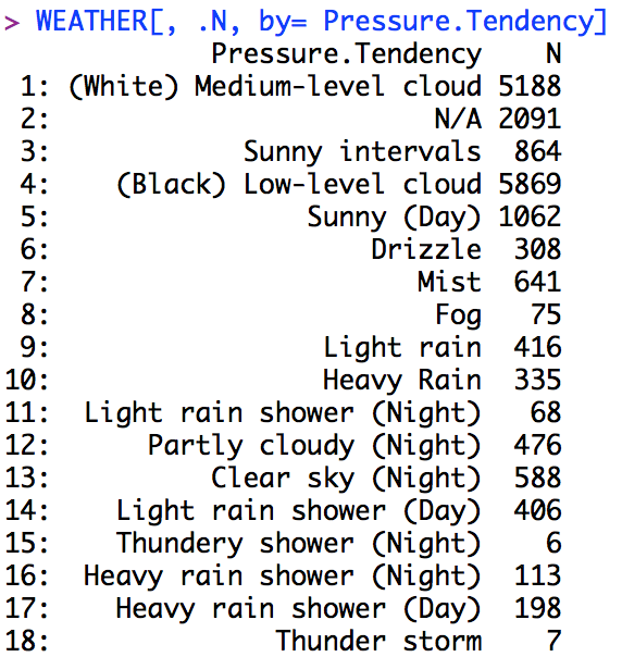
In addition, the data provides the temperature, wind speed and pressure. I construct a variable that measures the number of hours in which the weather was classified as “Heavy Rain” or  involved “Thunder”. Similarly, I construct daily averages of temperature.

Matching Local Authority Districts to weather points. As indicated, the weather data leaves a lot of room for improvement due to its coarseness and if you have any further data suggestions, let me know. I assign a weather observation, for which I have the latitude and longitude to the centroid of the nearest Local Authority District. I obtained a shapefile of Local Authority Districts covering just England.

Did the weather affect the referendum? There are at least two margins. First, the weather could affect turn out, as suggested above. Second, the weather could affect the mood. Lastly, the weather could have no effect overall.

Did the weather affect turnout? Probably not. The first set of regressions just explores the number of hours it rained during the day, the number of hours it rained in the morning and afternoon/ evening, the last puts both together. Further, I include the average temperature as regressor. Also, I include for Region fixed effect and the regressions are estimated just off English data, for which I could match the data to a shapefile. Throughout, no statistical association between rainfall and turnout appears in the data. This being said, the rainfall proxy is very crude, while temperature is more precisely measured. And here is at least a weak association suggesting that a 1 degree increase in mean temperature, reduced turnout by 0.35 percentage points. But the coefficient is too imprecise for any meaningful association.

summary(felm(Pct_Turnout ~ rainingcommuting23 + rainingnoncommuting23+ temp23 | Region | 0 | id, data=MERGED))
## 
## Call:
##    felm(formula = Pct_Turnout ~ rainingcommuting23 + rainingnoncommuting23 +      temp23 | Region | 0 | id, data = MERGED) 
## 
## Residuals:
##       Min        1Q    Median        3Q       Max 
## -0.142857 -0.026002  0.003213  0.027800  0.127797 
## 
## Coefficients:
##                        Estimate Cluster s.e. t value Pr(>|t|)
## rainingcommuting23    -0.001257     0.002663  -0.472    0.637
## rainingnoncommuting23  0.001951     0.002007   0.972    0.332
## temp23                -0.003253     0.002660  -1.223    0.222
## 
## Residual standard error: 0.04087 on 308 degrees of freedom
##   (62 observations deleted due to missingness)
## Multiple R-squared(full model): 0.3352   Adjusted R-squared: 0.3114 
## Multiple R-squared(proj model): 0.008567   Adjusted R-squared: -0.02684 
## F-statistic(full model, *iid*):14.12 on 11 and 308 DF, p-value: < 2.2e-16 
## F-statistic(proj model): 0.7966 on 3 and 308 DF, p-value: 0.4965

We can perform a type of placebo, by checking whether weather conditions on the day before the referendum had an effect. The only coefficient that gets anywhere close is rainfall during commuting hours on the day before. But again, there is a lack of precision. In any case, ideally finer data at the polling station level in addition to finer weather data is needed.

summary(felm(Pct_Turnout ~ rainingcommuting22 + rainingnoncommuting22+ temp22 | Region | 0 | id, data=MERGED))
## 
## Call:
##    felm(formula = Pct_Turnout ~ rainingcommuting22 + rainingnoncommuting22 +      temp22 | Region | 0 | id, data = MERGED) 
## 
## Residuals:
##       Min        1Q    Median        3Q       Max 
## -0.154669 -0.026714  0.003494  0.028441  0.115703 
## 
## Coefficients:
##                         Estimate Cluster s.e. t value Pr(>|t|)
## rainingcommuting22     4.440e-03    3.680e-03   1.207    0.229
## rainingnoncommuting22 -1.467e-05    2.594e-03  -0.006    0.995
## temp22                 4.816e-04    9.895e-04   0.487    0.627
## 
## Residual standard error: 0.04091 on 308 degrees of freedom
##   (62 observations deleted due to missingness)
## Multiple R-squared(full model): 0.3338   Adjusted R-squared:  0.31 
## Multiple R-squared(proj model): 0.006468   Adjusted R-squared: -0.02902 
## F-statistic(full model, *iid*):14.03 on 11 and 308 DF, p-value: < 2.2e-16 
## F-statistic(proj model): 0.7678 on 3 and 308 DF, p-value: 0.5128

Did the weather affect voting behavior?
There is a bit more here, the below regression suggest that higher temperatures were correlated with a higher percentage for the vote leave campaign. The turnout regressions suggested a potentially weakly lower turn out, as temperatures are higher. So did high temperatures induce Bremain voters to vote for Brexit?

The point estimate on temperature “temp23” significant at the 5% level, suggesting that a 1 degree increase in the temperature increased Brexit votes by 1 percentage point. This is a lot, but could just be a false positive – i.e. a statistical error. Nevertheless, maybe thats why there is so much to #Bregret? Did the heat of the moment induce voters to make a decision that they now regret?

summary(felm(Pct_Leave ~ rainingcommuting23 + rainingnoncommuting23+ temp23 | Region | 0 | id, data=MERGED))
## 
## Call:
##    felm(formula = Pct_Leave ~ rainingcommuting23 + rainingnoncommuting23 +      temp23 | Region | 0 | id, data = MERGED) 
## 
## Residuals:
##      Min       1Q   Median       3Q      Max 
## -30.9663  -5.2630   0.1153   5.8665  27.1071 
## 
## Coefficients:
##                       Estimate Cluster s.e. t value Pr(>|t|)  
## rainingcommuting23     -0.5980       0.4794  -1.248   0.2132  
## rainingnoncommuting23  -0.3900       0.3903  -0.999   0.3185  
## temp23                  1.1350       0.4935   2.300   0.0221 *
## ---
## Signif. codes:  0 '***' 0.001 '**' 0.01 '*' 0.05 '.' 0.1 ' ' 1
## 
## Residual standard error: 8.104 on 308 degrees of freedom
##   (62 observations deleted due to missingness)
## Multiple R-squared(full model): 0.3729   Adjusted R-squared: 0.3505 
## Multiple R-squared(proj model): 0.0276   Adjusted R-squared: -0.007127 
## F-statistic(full model, *iid*):16.65 on 11 and 308 DF, p-value: < 2.2e-16 
## F-statistic(proj model):  2.47 on 3 and 308 DF, p-value: 0.06201

In order to gain a bit more confidence, we can check whether the weather conditions on the day before. Throughout, there is no indication that this was the case (see below).

summary(felm(Pct_Leave ~ rainingcommuting22 + rainingnoncommuting22+ temp22 | Region | 0 | id, data=MERGED))
## 
## Call:
##    felm(formula = Pct_Leave ~ rainingcommuting22 + rainingnoncommuting22 +      temp22 | Region | 0 | id, data = MERGED) 
## 
## Residuals:
##      Min       1Q   Median       3Q      Max 
## -31.3071  -5.0842   0.5469   5.2357  30.5874 
## 
## Coefficients:
##                       Estimate Cluster s.e. t value Pr(>|t|)
## rainingcommuting22      0.4547       0.7448   0.610    0.542
## rainingnoncommuting22  -0.2837       0.5679  -0.500    0.618
## temp22                  0.1565       0.3447   0.454    0.650
## 
## Residual standard error: 8.208 on 308 degrees of freedom
##   (62 observations deleted due to missingness)
## Multiple R-squared(full model): 0.3567   Adjusted R-squared: 0.3338 
## Multiple R-squared(proj model): 0.00249   Adjusted R-squared: -0.03314 
## F-statistic(full model, *iid*):15.53 on 11 and 308 DF, p-value: < 2.2e-16 
## F-statistic(proj model): 0.211 on 3 and 308 DF, p-value: 0.8888

What can we take from this?I was concinced that I could document an effect of rainfall during the commuting hours. Having experienced the Waterloo commute for a year, I could sympathize with the idea of not going to vote after a long day and a terrible commute. The retired can go vote any time during the day, why the commuters/ employed need to arrange this for the evening or mornign hours. Is this fair or de-facto disenfranchising a set of voters? With the crude data on rainfall, I do not find any evidence in support of the rainfall channel. This would have been policy relevant.

The temperature regressions indicate some weak evidence on voting behavior, suggesting higher Brexit vote share, but no statistically discernible effect on turn out.

There are a lot of buts and ifs here. The analysis is super coarse, but potentially with finer polling data, an actual analysis of commuting flows and better weather data, some points could be driven home.

Maybe that is just my attempt to cope with the Brexit shock. As a German living and working in the UK, I am quite shocked and devastated and worried about what the future holds for me, my partner and my friends here.

Thiemo Fetzer, Assistant Professor in Economics, University of Warwick.

Dropbox Link with all data and code


Correction For Spatial And Temporal Auto-Correlation In Panel Data: Using R To Estimate Spatial HAC Errors Per Conley

Darin Christensen and Thiemo Fetzer


tl;dr: Fast computation of standard errors that allows for serial and spatial auto-correlation.


Economists and political scientists often employ panel data that track units (e.g., firms or villages) over time. When estimating regression models using such data, we often need to be concerned about two forms of auto-correlation: serial (within units over time) and spatial (across nearby units). As Cameron and Miller (2013) note in their excellent guide to cluster-robust inference, failure to account for such dependence can lead to incorrect conclusions: “[f]ailure to control for within-cluster error correlation can lead to very misleadingly small standard errors…” (p. 4).

Conley (1999, 2008) develops one commonly employed solution. His approach allows for serial correlation over all (or a specified number of) time periods, as well as spatial correlation among units that fall within a certain distance of each other. For example, we can account for correlated disturbances within a particular village over time, as well as between that village and every other village within one hundred kilometers. As with serial correlation, spatial correlation can be positive or negative. It can be made visually obvious by plotting, for example, residuals after removing location fixed effects.

Example Visualization of Spatial Correlation
Example Visualization of Spatial Correlation from Radil, S. Matthew, Spatializing Social Networks: Making Space for Theory In Spatial Analysis, 2011.

We provide a new function that allows R users to more easily estimate these corrected standard errors. (Solomon Hsiang (2010) provides code for STATA, which we used to test our estimates and benchmark speed.) Moreover using the excellent lfe, Rcpp, and RcppArmadillo packages (and Tony Fischetti’s Haversine distance function), our function is roughly 20 times faster than the STATA equivalent and can scale to handle panels with more units. (We have used it on panel data with over 100,000 units observed over 6 years.)

This demonstration employs data from Fetzer (2014), who uses a panel of U.S. counties from 1999-2012. The data and code can be downloaded here.


STATA Code:

We first use Hsiang’s STATA code to compute the corrected standard errors (spatHAC in the output below). This routine takes just over 25 seconds.

cd "~/Dropbox/ConleySEs/Data"
clear; use "new_testspatial.dta"

tab year, gen(yy_)
tab FIPS, gen(FIPS_)

timer on 1
ols_spatial_HAC EmpClean00 HDD yy_*FIPS_2-FIPS_362, lat(lat ) lon(lon ) t(year) p(FIPS) dist(500) lag(5) bartlett disp

# *-----------------------------------------------
# *    Variable |   OLS      spatial    spatHAC
# *-------------+---------------------------------
# *         HDD |   -0.669     -0.669     -0.669
# *             |    0.608      0.786      0.838

timer off 1
timer list 1
#  1:     24.8 /        3 =      8.2650

R Code:

Using the same data and options as the STATA code, we then estimate the adjusted standard errors using our new R function. This requires us to first estimate our regression model using the felm function from the lfe package.

# Loading sample data:
dta_file <- "~/Dropbox/ConleySEs/Data/new_testspatial.dta"
DTA <-data.table(read.dta(dta_file))
setnames(DTA, c("latitude", "longitude"), c("lat", "lon"))

# Loading R function to compute Conley SEs:
source("~/Dropbox/ConleySEs/ConleySEs_17June2015.R")

ptm <-proc.time()

# We use the felm() from the lfe package to estimate model with year and county fixed effects.
# Two important points:
# (1) We specify our latitude and longitude coordinates as the cluster variables, so that they are included in the output (m).
# (2) We specify keepCx = TRUE, so that the centered data is included in the output (m).

m <-felm(EmpClean00 ~HDD -1 |year +FIPS |0 |lat +lon,
  data = DTA[!is.na(EmpClean00)], keepCX = TRUE)

coefficients(m) %>%round(3) # Same as the STATA result.
   HDD 
-0.669 

We then feed this model to our function, as well as the cross-sectional unit (county FIPS codes), time unit (year), geo-coordinates (lat and lon), the cutoff for serial correlation (5 years), the cutoff for spatial correlation (500 km), and the number of cores to use.

SE <-ConleySEs(reg = m,
    unit = "FIPS", 
    time = "year",
    lat = "lat", lon = "lon",
    dist_fn = "SH", dist_cutoff = 500, 
    lag_cutoff = 5,
    cores = 1, 
    verbose = FALSE) 

sapply(SE, sqrt) %>%round(3) # Same as the STATA results.
        OLS     Spatial Spatial_HAC 
      0.608       0.786       0.837 
proc.time() -ptm
   user  system elapsed 
  1.619   0.055   1.844 

Estimating the model and computing the standard errors requires just over 1 second, making it over 20 times faster than the comparable STATA routine.


R Using Multiple Cores:

Even with a single core, we realize significant speed improvements. However, the gains are even more dramatic when we employ multiple cores. Using 4 cores, we can cut the estimation of the standard errors down to around 0.4 seconds. (These replications employ the Haversine distance formula, which is more time-consuming to compute.)

pkgs <-c("rbenchmark", "lineprof")
invisible(sapply(pkgs, require, character.only = TRUE))

bmark <-benchmark(replications = 25,
  columns = c('replications','elapsed','relative'),
  ConleySEs(reg = m,
    unit = "FIPS", time = "year", lat = "lat", lon = "lon",
    dist_fn = "Haversine", lag_cutoff = 5, cores = 1, verbose = FALSE),
  ConleySEs(reg = m,
    unit = "FIPS", time = "year", lat = "lat", lon = "lon",
    dist_fn = "Haversine", lag_cutoff = 5, cores = 2, verbose = FALSE),
  ConleySEs(reg = m,
    unit = "FIPS", time = "year", lat = "lat", lon = "lon",
    dist_fn = "Haversine", lag_cutoff = 5, cores = 4, verbose = FALSE))
bmark %>%mutate(avg_eplased = elapsed /replications, cores = c(1, 2, 4))
  replications elapsed relative avg_eplased cores
1           25   23.48    2.095      0.9390     1
2           25   15.62    1.394      0.6249     2
3           25   11.21    1.000      0.4483     4

Given the prevalence of panel data that exhibits both serial and spatial dependence, we hope this function will be a useful tool for applied econometricians working in R.


Feedback Appreciated: Memory vs. Speed Tradeoff

This was Darin’s first foray into C++, so we welcome feedback on how to improve the code. In particular, we would appreciate thoughts on how to overcome a memory vs. speed tradeoff we encountered. (You can email Darin at darinc[at]stanford.edu.)

The most computationally intensive chunk of our code computes the distance from each unit to every other unit. To cut down on the number of distance calculations, we can fill the upper triangle of the distance matrix and then copy it to the lower triangle. With [math]N[/math] units, this requires only  [math](N (N-1) /2)[/math] distance calculations.

However, as the number of units grows, this distance matrix becomes too large to store in memory, especially when executing the code in parallel. (We tried to use a sparse matrix, but this was extremely slow to fill.) To overcome this memory issue, we can avoid constructing a distance matrix altogether. Instead, for each unit, we compute the vector of distances from that unit to every other unit. We then only need to store that vector in memory. While that cuts down on memory use, it requires us to make twice as many   [math](N (N-1))[/math]  distance calculations.

As the number of units grows, we are forced to perform more duplicate distance calculations to avoid memory constraints – an unfortunate tradeoff. (See the functions XeeXhC and XeeXhC_Lg in ConleySE.cpp.)


sessionInfo()
R version 3.2.2 (2015-08-14)
Platform: x86_64-apple-darwin13.4.0 (64-bit)
Running under: OS X 10.10.4 (Yosemite)

locale:
[1] en_GB.UTF-8/en_GB.UTF-8/en_GB.UTF-8/C/en_GB.UTF-8/en_GB.UTF-8

attached base packages:
[1] stats     graphics  grDevices utils     datasets  methods  
[7] base     

other attached packages:
 [1] RcppArmadillo_0.5.400.2.0 Rcpp_0.12.0              
 [3] geosphere_1.4-3           sp_1.1-1                 
 [5] lfe_2.3-1709              Matrix_1.2-2             
 [7] ggplot2_1.0.1             foreign_0.8-65           
 [9] data.table_1.9.4          dplyr_0.4.2              
[11] knitr_1.11               

loaded via a namespace (and not attached):
 [1] Formula_1.2-1    magrittr_1.5     MASS_7.3-43     
 [4] munsell_0.4.2    xtable_1.7-4     lattice_0.20-33 
 [7] colorspace_1.2-6 R6_2.1.1         stringr_1.0.0   
[10] plyr_1.8.3       tools_3.2.2      parallel_3.2.2  
[13] grid_3.2.2       gtable_0.1.2     DBI_0.3.1       
[16] htmltools_0.2.6  yaml_2.1.13      assertthat_0.1  
[19] digest_0.6.8     reshape2_1.4.1   formatR_1.2     
[22] evaluate_0.7.2   rmarkdown_0.8    stringi_0.5-5   
[25] compiler_3.2.2   scales_0.2.5     chron_2.3-47    
[28] proto_0.3-10    

Stacking Regressions: Latex Tables with R and stargazer

In my paper on the impact of the shale oil and gas boom in the US, I run various instrumental variables specifications. For these, it is nice to stack the regression results one on the other – in particular, to have one row for the IV results, one row for the Reduced Form and maybe one row for plain OLS to see how the IV may turn coefficients around.

I found that as of now – there is no way to do that directly; please correct me if I am wrong.

The layout I have in mind is as in the screenshot of my table.

Sample Table with Stacked Regression Results In Stata, this can be accomplished through the use of esttab with the fragment, and append feature. This appends successive rows to an existing table and you can label the rows using the “refcat” option.

However, in R this is not possible as of yet. I have mainly worked with stargazer, as Marek has added felm objects for high dimensional fixed effects to be handled by his stargazer package.

The following functions are a “hack” that extracts the particular rows from the generated latex code by the stargazer package.

You can then piece the table together by combining the individual elements. The idea is that you have a single stargazer command that is passed to the various functions that extract the different features. Obviuously, this can be done a lot more elegant as the code is extremely hacky, but it does work

Marek has said that he is thinking of incorporating a stacking option into stargazer, but for now, my hack works reasonably well. The key thing to realise is that stargazer calls have the option to return

The following character strings can be used in the table.layout and omit.table.layout arguments of the stargazer command.

“-“ single horizontal line
“=” double horizontal line
“-!” mandatory single horizontal line
“=!” mandatory double horizontal line
“l” dependent variable caption
“d” dependent variable labels
“m” model label
“c” column labels
“#” model numbers
“b” object names
“t” coefficient table
“o” omitted coefficient indicators
“a” additional lines
“n” notes
“s” model statistics


The following functions will simply extract the rows that are being returned.

stargazer.keepcolnums<-function(call="") {
command<-gsub("\\)$",", table.layout='#'\\)",command)
call<-eval(parse(text=command))
bounds<-grep("tabular",call)
row1<- call[(bounds[1]+1):(bounds[2]-1)]
row1<-gsub("^\\\\\\\\\\[-1\\.8ex\\]\\\\hline $", "", row1)
row1<-gsub("^\\\\hline \\\\\\\\\\[-1\\.8ex\\] $","",row1)
row1<-row1[row1!=""]
}
stargazer.keeprow<-function(call="") {
command<-gsub("\\)$",", table.layout='t'\\)",command)
call<-eval(parse(text=command))
bounds<-grep("tabular",call)
row1<- call[(bounds[1]+1):(bounds[2]-1)]
row1<-gsub("^\\\\\\\\\\[-1\\.8ex\\]\\\\hline $", "", row1)
row1<-gsub("^\\\\hline \\\\\\\\\\[-1\\.8ex\\] $","",row1)
row1<-row1[row1!=""]
}

stargazer.keepstats<-function(call="") {
command<-gsub("\\)$",", table.layout='s'\\)",command)
call<-eval(parse(text=command))
row1<-gsub("(.*)\\\\\\\\\\[-1\\.8ex\\](.*)(\\\\end\\{tabular\\})(.*)","\\2",paste(call,collapse=" "))
row1
}
stargazer.begintable<-function(call="") {
command<-gsub("\\)$",", table.layout='m'\\)",command)
call<-eval(parse(text=command))
row1<-paste("\\begin{tabular}",gsub("(.*)\\\\begin\\{tabular\\}(.*)(\\\\end\\{tabular\\})(.*)","\\2",paste(call,collapse="\n")),sep="")
row1
}
stargazer.varlabels<-function(call="") {
command<-gsub("\\)$",", table.layout='d'\\)",command)
call<-eval(parse(text=command))
row1<-paste("\\begin{tabular}",gsub("(.*)\\\\begin\\{tabular\\}(.*)(\\\\end\\{tabular\\})(.*)","\\2",paste(call,collapse="\n")),sep="")
row1
}

stargazer.keepcollabels<-function(call="") {
command<-gsub("\\)$",", table.layout='c'\\)",command)
call<-eval(parse(text=command))
row1<-gsub("(.*)\\\\\\\\\\[-1\\.8ex\\](.*)(\\\\end\\{tabular\\})(.*)","\\2",paste(call,collapse=" "))
row1
}

stargazer.keepomit<-function(call="") {
command<-gsub("\\)$",", table.layout='o'\\)",command)
call<-eval(parse(text=command))
row1<-gsub("(.*)\\\\\\\\\\[-1\\.8ex\\](.*)(\\\\end\\{tabular\\})(.*)","\\2",paste(call,collapse="\n"))
row1
}

It easiest to see how you can use these functions to construct stacked regression output by giving a simple example.

###the global command to be passed to the hacky ###functions that extract the individual bits
## OLS is a list of OLS results from running the
## lfe command
command<-'stargazer(OLS , keep=c("post08shale:directutilityshare","post08shale"), covariate.labels=c("Energy Intensity x Shale","Shale"), header=FALSE, out.header=FALSE, keep.stat=c("n","adj.rsq"))'

begintable<-stargazer.begintable(command)
###some multicolumn to combine 
collcombine<-c("& \\multicolumn{4}{c}{Tradable Goods Sector Only} & \\multicolumn{3}{c}{Additional Sectors} & \\cmidrule(lr){2-5} \\cmidrule(lr){6-8}")
collabel<-stargazer.keepcollabels(command)
colnums<-stargazer.keepcolnums(command)
##plain OLS row
row1<-stargazer.keeprow(command)
##the stats part for the OLS (number of Obs, R2)
stats<-stargazer.keepstats(command)
##the rows for the Fixed effect indicators
omitted<-stargazer.keepomit(command)

##the IV command passing a list of IV results in ## IV object
command<-'stargazer(IV , keep=c("post08anywell:directutilityshare","post08anywell"), covariate.labels=c("Energy Intensity x Anywell","Anywell"), header=FALSE, out.header=FALSE, keep.stat=c("n","adj.rsq"))'

##IV row
row2<-stargazer.keeprow(command)
footer<-c("\\end{tabular}\n" )

###now combine all the items
cat(begintable,collcombine,collabel,colnums,"\\hline \\\\\\emph{Reduced Form} \\\\",row1,""\\hline \\\\\\emph{Reduced Form} \\\\",row2,stats,"\\hline\\hline",footer, file="Draft/tables/energyintensity.tex", sep="\n")

I know the solution is a bit hacky, but it works and does the trick.


Fracking and House Prices on the Marcellus Shale

Starting last summer I worked on a short project that set out to estimate the potential costs of externalities due to unconventional shale gas production in the Marcellus shale on local house prices using a dataset of roughly 150,000 recently sold houses in Ohio, West Virginia and Pennsylvania.

The data suggests that proximity to a natural gas well is correlated with lower housing prices, which confirms previous studies.

fracking-houseprices

I stopped working on a project that looks at the impact of nearby shale gas extraction on property prices for the Marcellus shale. Instead, I focused on my paper “Fracking Growth” that evaluates the employment consequences of the shale oil and gas boom in the US more generally.

Everybody can have a look at the data and the document as it stands on sharelatex, where I also tried Sharelatex’s Knitr capacities, which are still somewhat limited as a lot of R-packages I usually work with are not yet installed.

The public sharelatex file, the data and the R script can be accessed here:

https://www.sharelatex.com/project/534d232b32ed2b25466b2541?r=6f73efc4&rs=ps&rm=d

Here are some preliminary snippets. The data used in this study comes from Zillow.com In Fall 2013 I downloaded data for recently sold houses. I focused the download to cover all or most of the counties that are somewhat near the Marcellus shale in West Virginia, Ohio and Pennsylvania. This list goes back to 2011 and provides data for 151,156 sold properties.

load(file = "HOUSES.rdata")
library(xtable)
table(HOUSES$year)
####  2011  2012  2013
#### 40087 63248 47821

A simple tabulation suggests that most data is for 2012.

Some characteristics that are included in the data are the sale price in USD, the number of bedrooms, number of bathrooms, the built up land size in square feet, the year the property was built and for some properties also the lot size.

The properties have geo-coordinates, which are used to intersect the location of the property with census-tract shapefiles. This will allow the adding of further characteristics at the census-tract level to control for general local characteristics.

The geo-coordinates are further used to compute the exact distance of a property to the nearest actual or permitted well in the year that the property was sold. Distances are computed in meters by computing the Haversine distance on a globe with radius r = 6378137 meters.

The following graph plots the average price per square foot as a function of distance to the nearest well in the year in which the property was sold. I group distances into 500 meter bins.

plot(HOUSES[, list(soldprice =sum(soldprice)/sum(sqft)), by=distancecat ], xlab="Distance to Well", ylab="Price per sqft")

A first inspection suggests a positive gradient in distance, that is – however, quite non-monotone.

Non-monotonic relationship between distance to the nearest oil or gas well and price per sqft.

Does this relationship hold up when running a hedonic pricing regression?

[math]log(y_{ict}) = \gamma \times welldistance_{i} + \beta \times X_i + a_c + \eta_t + e_{ict}[/math]

These are estimated using the lfe package, as I introduce quite demanding fixed effects (census-tract and county by year). The lfe package takes these fixed effects out iteratively before running the actual regression on the demeaned data.

The results for two chosen bandwidths are presented in the table below. There appears to be a positive gradient – being further away from a well correlates with higher prices per square foot.

Regression results comparing sold houses nearby unconventional gas wells on the Marcellus shale

Clearly, the important question is whether one can separate out the property price appreciation that is likely to happen due to the local economic boom from the price differentials that may arise due to the presence of the local externalities and whether, one can separate out externalities due to environmental degradation as distinct from price differentials arising due to factors discussed in the beginning: no access to mortgage lending or insurances.

Unfortunately, I do not have the time to spend more time on this now, but I think a short paper is still feasible…


Regressions with Multiple Fixed Effects – Comparing Stata and R

In my paper on the impact of the recent fracking boom on local economic outcomes, I am estimating models with multiple fixed effects. These fixed effects are useful, because they take out, e.g. industry specific heterogeneity at the county level – or state specific time shocks.

The models can take the form:

[math]y_{cist} = \alpha_{ci} + b_{st} + \gamma_{it}+ X_{cist}'\beta + \epsilon_{cist}[/math]  

where [math]\alpha_{ci}[/math] is a set of county-industry, [math]b_{ci}[/math] a set of state-time and [math]\gamma_{it}[/math] is a set of industry-time fixed effects.

Such a specification takes out arbitrary state-specific time shocks and industry specific time shocks, which are particularly important in my research context as the recession hit tradable industries more than non-tradable sectors, as is suggested in Mian, A., & Sufi, A. (2011). What Explains High Unemployment ? The Aggregate Demand Channel.

How can we estimate such a specification?
Running such a regression in R with the lm or reg in stata will not make you happy, as you will need to invert a huge matrix. An alternative in Stata is to absorb one of the fixed-effects by using xtreg or areg. However, this still leaves you with a huge matrix to invert, as the time-fixed effects are huge; inverting this matrix will still take ages.

However, there is a way around this by applying the Frisch-Waugh Lovell theorem iteratively (remember your Econometrics course?); this basically means you iteratively take out each of the fixed effects in turn by demeaning the data by that fixed effect. The iterative procedure is described in detail in Gaure (2013), but also appears in Guimaraes and Portugal(2010).

Simen Gaure has developed an R-package called lfe, which performs the demeaning for you and also provides the possibility to run instrumental variables regressions; it theoretically supports any dimensionality of fixed effects. The key benefit of Simen Gaure’s implementation is the flexibility, the use of C in the background for some of the computing and its support for multicore processing, which speeds up the demeaning process dramatically, especially the larger your samples get..

In Stata there is a package called reg2hdfe and reg3hdfe which has been developed by Guimaraes and Portugal (2010). As the name indicates, these support only fixed effects up to two or three dimensions.

Lets see how – on the same dataset – the runtimes of reg2hdfe and lfe compare.

Comparing Performance of Stata and R

I am estimating the following specification

[math]y_{cist} = \alpha_{ci} + b_{sit} + \gamma_{it}+ X_{cist}'\beta + \epsilon_{cist}[/math]  

where [math]\alpha_{ci}[/math] is a set of county-industry, [math]b_{ci}[/math] a set of state-time fixed effects. There are about 3000 counties in the dataset and 22 industries. Furthermore, there are 50 states and the time period is also about 50 quarters. This means – in total – there are 3000 x 22 = 66,000 county-industry fixed effects to be estimated and 22 x 50 x 50 = 55,000 time fixed effects to be estimated. The sample I work with has sufficient degrees of freedom to allow the estimation of such a specification – I work with roughly 3.7 million observations.

I have about 10 covariates that are in [math]X_{cist}[/math], i.e. these are control variables that vary within county x industry over state x industry x time.

Performance in Stata

In order to time the length of a stata run, you need to run
set rmsg on, which turns on a timer for each command that is run.

The command I run in stata is

reg2hdfe logy x1-x10,  id1(sitq ) id2(id) cluster(STATE_FIPS )

You should go get a coffee, because this run is going to take quite a bit of time. In my case, it took t=1575.31, or just about 26 minutes.

Performance in R 
In order to make the runs of reg2hdfe and lfe, we need to set the tolerance level of the convergence criterion to be the same in both. The standard tolerance in Stata is set at $$1e^{-6}$$, while for lfe package it is set at $$1e^{-8}$$. In order to make the runs comparable you can set the options in the R package lfe options explicitly:

options(lfe.eps=1e-6)

The second change we need to make is to disallow lfe to use multiple cores, since reg2hdfe uses only a single thread. We can do this by setting:

options(lfe.threads=1)

Now lets run this in R using:

system.time(summary(felm(log(y) ~ x1 + x2 +x3 +x4 + x5 + x6 + x7 +x8 + x9 + x10 + G(id)+G(sitq),
data=EMP, cluster=c("STATE_FIPS"))))

The procedure converges in a lot quicker than Stata…

 user system elapsed 
208.450 23.817 236.831 

It took a mere 4 minutes. Now suppose I run this in four separate threads…

user system elapsed 
380.964 23.540 177.520


Running this on four threads saves about one minute in processing time; not bad, but not too much gained; the gains from multi-threading increase, the more fixed-effects are added and the larger the samples are.