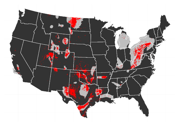
Starting last summer I worked on a short project that set out to estimate the potential costs of externalities due to unconventional shale gas production in the Marcellus shale on local house prices using a dataset of roughly 150,000 recently sold houses in Ohio, West Virginia and Pennsylvania.
The data suggests that proximity to a natural gas well is correlated with lower housing prices, which confirms previous studies.
I stopped working on a project that looks at the impact of nearby shale gas extraction on property prices for the Marcellus shale. Instead, I focused on my paper “Fracking Growth” that evaluates the employment consequences of the shale oil and gas boom in the US more generally.
Everybody can have a look at the data and the document as it stands on sharelatex, where I also tried Sharelatex’s Knitr capacities, which are still somewhat limited as a lot of R-packages I usually work with are not yet installed.
The public sharelatex file, the data and the R script can be accessed here:
https://www.sharelatex.com/project/534d232b32ed2b25466b2541?r=6f73efc4&rs=ps&rm=d
Here are some preliminary snippets. The data used in this study comes from Zillow.com In Fall 2013 I downloaded data for recently sold houses. I focused the download to cover all or most of the counties that are somewhat near the Marcellus shale in West Virginia, Ohio and Pennsylvania. This list goes back to 2011 and provides data for 151,156 sold properties.
load(file = "HOUSES.rdata")
library(xtable)
table(HOUSES$year)
####  2011  2012  2013
#### 40087 63248 47821
A simple tabulation suggests that most data is for 2012.
Some characteristics that are included in the data are the sale price in USD, the number of bedrooms, number of bathrooms, the built up land size in square feet, the year the property was built and for some properties also the lot size.
The properties have geo-coordinates, which are used to intersect the location of the property with census-tract shapefiles. This will allow the adding of further characteristics at the census-tract level to control for general local characteristics.
The geo-coordinates are further used to compute the exact distance of a property to the nearest actual or permitted well in the year that the property was sold. Distances are computed in meters by computing the Haversine distance on a globe with radius r = 6378137 meters.
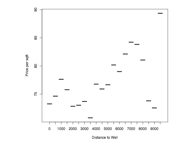
The following graph plots the average price per square foot as a function of distance to the nearest well in the year in which the property was sold. I group distances into 500 meter bins.
plot(HOUSES[, list(soldprice =sum(soldprice)/sum(sqft)), by=distancecat ], xlab="Distance to Well", ylab="Price per sqft")
A first inspection suggests a positive gradient in distance, that is – however, quite non-monotone.

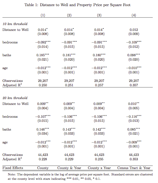
Does this relationship hold up when running a hedonic pricing regression?
[math]log(y_{ict}) = \gamma \times welldistance_{i} + \beta \times X_i + a_c + \eta_t + e_{ict}[/math]
These are estimated using the lfe package, as I introduce quite demanding fixed effects (census-tract and county by year). The lfe package takes these fixed effects out iteratively before running the actual regression on the demeaned data.
The results for two chosen bandwidths are presented in the table below. There appears to be a positive gradient – being further away from a well correlates with higher prices per square foot.

Clearly, the important question is whether one can separate out the property price appreciation that is likely to happen due to the local economic boom from the price differentials that may arise due to the presence of the local externalities and whether, one can separate out externalities due to environmental degradation as distinct from price differentials arising due to factors discussed in the beginning: no access to mortgage lending or insurances.
Unfortunately, I do not have the time to spend more time on this now, but I think a short paper is still feasible…

I’m impressed by your blog quality. I have two specific questions: how did you get all these house prices through Zillow, and how did you find the geo coordinates of these addresses? I was under the impression that finding the geolocation of 100 000 addresses was hard.
The data is from Zillow.com, there is a way you can zoom in to an area and browse the recently sold houses. The houses are displayed on the map, see on e.g. on http://www.zillow.com/homes/recently_sold/Bradford-County-PA/2149_rid/days_sort/42.012571,-76.069336,41.532226,-76.974335_rect/9_zm/.
You can then write a script to grab the information about the houses displayed on the map and this information contains the geo-coordinates as well.
Thanks for the post Thiemo. I am trying to replicate your results for an unrelated project on pricing houses in the USA. Is there any way you could post your R workspace?
Thanks,
Jamie
Dear Jamie,
unfortunately I dont really have the stuff around handy right now. Somebody seems to have broken the sharelatex document I think.
If I get back to it at some point, I will let you know.
Best Thiemo