In my recent research I have worked on understanding the key correlates of Brexit. This paper is joint work with my co-authors Sascha Becker and Dennis Novy and has now been published in Economic Policy. After having gone through the peer-review process, I am very happy to share the data and the underlying code.
On the construction of a rich local authority level dataset
After the EU Referendum, I started working on assembling a dataset to study the question to what extent low turnout among potential remain voters may help to understand the result of the referendum. In particular, back then I looked at the extent to which rainfall may have discouraged people to turn up to vote in the first place. After all, a lot of polls, the financial markets and betting markets seemed to indicate that Remain would win.
It was not inconceivable to imagine that turnout may have been particularly low among a set of voters living in the London commuter belt, who were turned off from voting on a working day after an arduous journey into London that was marred by train cancelations due to the bad weather.
The result then was that there appears to have been a weak effect on turnout, but this effect was not biased in either direction with regard to voter preferences: Remain would have lost also on a sunny day (we confirm this finding in the new paper with a different rainfall data set).
In any case, this was the starting point to a significant data collection effort. In particular we have combined data from all the 380 local authorities in England, Scotland and Wales as well as some data of ward level voting across five cities. The resulting set of covariates is quite sizable and they can be roughly grouped into the following four categories:
- characteristics of the underlying economic structure of an area, like the unemployment rate, wages or sectoral employment shares and changes therein,
- demographic and human capital characteristics like age structure, education or life satisfaction,
- exposure to the EU measured by indicators like the level of EU transfers, trade and the growth rate of immigration from other EU countries,
- public service provision and fiscal consolidation that covers the share of public employment, as well as the reduction in public spending per capita among others and NHS performance metrics.
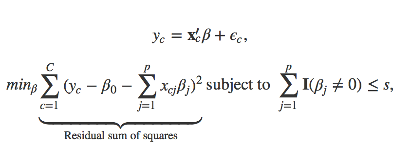
To analyse which of these covariates are strong correlates of the Leave vote share in an area, we used a simple machine-learning method that chooses the best subset of covariates that best predicts the referendum Leave share. The idea is to build a robust predictive model that could achieve significant out of sample prediction accurracy.
More formally, best subset selection solves the following optimization problem to obtain an optimal vector beta that can robustly predict the vote leave share y_c
While the formulation may be a bit technical, it boils down to estimating all possible ways to combine regressors. That means, all possible ways of estimating a model that includes 1, 2, 3, …, p covariates are being estimated. This amounts to estimating (2^p) models, which becomes infeasible to estimate very fast. Lasso and other methods such as forward- and backward stepwise selection are solving approximations to the combinatorical problem that BSS solves. The method is usually taught at the beginning of machine learning courses as it provides a great way to illustrate the bias-variance tradeoff.
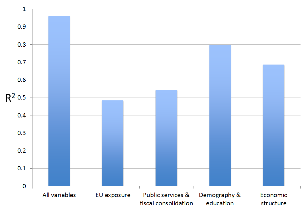
The result can be summarized in a simple bar chart and is somewhat striking:
What this suggests is that “Fundamental factors†such economic structure, demographics and human capital are strongest correlates of Leave vote in the UK; the direct level effects of migration and trade exposure captured in the group of regressors called “EU Exposure†seem second order.
Also what is striking that even very simple empirical models with just 10 – 20 variables are doing a good job in capturing the variation in the vote leave share across the whole of the UK. The best model that includes variables measuring vote shares of different parties (especially UKIP) from the 2014 European Parliamentary election captures 95% of the overall variation.
The observation that variables capturing direct exposure to the European Union, in particular, Immigration seems at odds with voter narratives around the EU referendum, which were doinated by the immigration topic. In fact, the 2015 British Election study suggests that voters considered immigration to be the single most important issue of the time.

In the above the word cloud the keyword immigration is just quite striking. Looking at the bigram word cloud drawn from the British Election study, the themes of the individual responses become even more apparent.

There things like “many people”, “small island”, “uncontrolled immigration” appear in addition to the simple immigration keyword. But also other themes, such as “national debt”, “health service” and concerns about the “welfare system” seem to feature quite large. Overall this suggests that immigration may have been a salient feature in the public debate, but it seems at odds with the fact that the variable groups pertaining to EU immigration seem to capture very little of the variation in the intensity of the leave vote across the UK.
In another paper with Sascha we confirm this observation  in a panel setup. We show that a local area’s exposure to Eastern European immigration has, at best, only a small impact on anti-EU preferences in the UK as measured by UKIP voting in European Parliamentary Elections.
While our code for the Economic policy paper is implemented in Stata, it is very easy to replicate this work in Stata. Below is an example of how you would implement BSS in R through the leaps package.
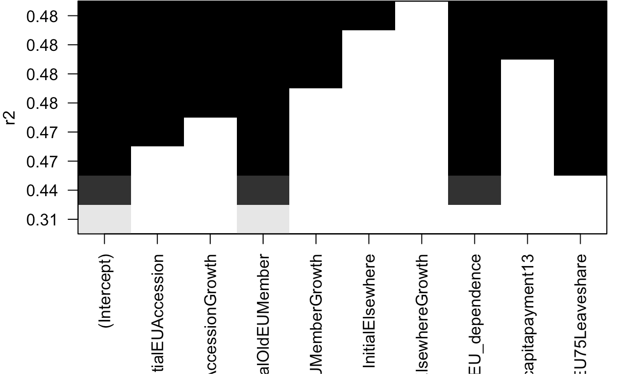
The leaps package has a nice visualization of which regressors are included in which of the best models. The below example replicates the results in our Table 1.
library(data.table)
library(haven)
library(leaps)
DTA<-data.table(read_dta(file="data/brexitevote-ep2017.dta"))

#TABLE 1 IN THE PAPER WOULD BE REPLICATED BY RUNNING
TABLE1<-regsubsets(Pct_Leave~InitialEUAccession+MigrantEUAccessionGrowth+InitialOldEUMember+MigrantOldEUMemberGrowth+InitialElsewhere+MigrantElsewhereGrowth+Total_EconomyEU_dependence+eufundspercapitapayment13+EU75Leaveshare,nbest=1,data=DTA)

plot(TABLE1,scale="r2")If you want to replicate the word clouds from the 2015 British Election study, the following lines of code will do. You will need to download the British Election Study dataset here.
library(data.table)
library(haven)
library(quanteda)

DTA<-data.table(read_dta(file="data/bes_f2f_original_v3.0.dta"))

C<-corpus(DTA$A1)
docnames(C)<-DTA$finalserialno

C.dfmunigram

C.dfmunigram <- dfm(C, tolower = TRUE, stem = FALSE, removeNumbers=TRUE,removePunct=TRUE, remove = stopwords("english"), ngrams=1)
C.dfm<-dfm(C, tolower = TRUE, stem = FALSE, removeNumbers=TRUE,removePunct=TRUE, remove = stopwords("english"), ngrams=2)

plot(C.dfmunigram)

plot(C.dfm)

this
