The Yemeni civil war has received very little attention despite the growing humanitarian disaster. There is a lack of reliable figures on the extent of the human suffering in Yemen. The few data that is available suggests that it is immense. According to the UN, from March 2015 to August 2016, over 10,000 people have been killed in Yemen, including 3,799 civilians.
This note asks whether high frequency satellite images do capture the extent to which conflict is ongoing in Yemen and asks in particular, whether there is distinct geographic variation suggesting which areas are most affected by the ongoing conflict.
Can the effect and the spatial incidence of the conflict in Yemen be traced through satellite images?
Satellite images have been used to study urban sprawl and general economic growth and development. The extent to which satellite images can be used to study man-made disasters such as conflicts is not widely explored.
There are lots of other papers that have used various night light data sets to study urbanization, ethnic favoritism, and economic growth (see Henderson et al, 2012 ; Michalopoulos and Papaioannou 2013,  Hodler and Raschky, 2014).
In related work Fetzer et al., 2016, I studied the extent to which light emissions in the early 1990s can be used to obtain a measure of the extent of power rationing in Colombia following El-Nino induced droughts. In another project, we use the DMSP night light images to study the evolution of cities over time and how democratization can change the relative distribution of cities Fetzer and Shanghavi, 2015.
Since 2012, the VIIRS
high frequency and high resolution satellite images capturing night lights emissions are available from NASA’s Earth Observation Group. They have now been made available for analysis on Google’s Earth Engine, making them much more accessible to the wider research audience.
Lets have a look at night light Yemen before and after the Saudi Arabian military intervention.
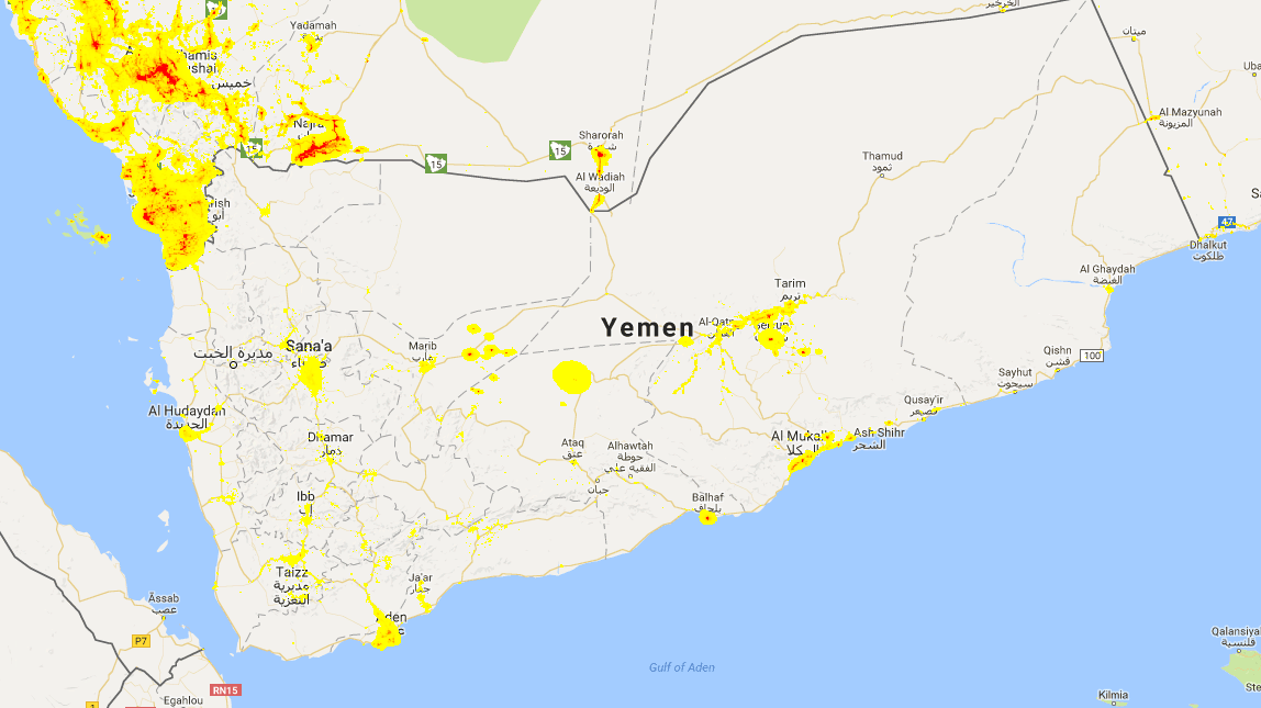
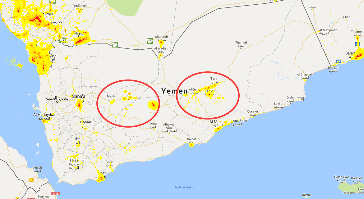
The light scales are identical, indicating that relative to the border with Saudi Arabia, the night light emissions from Yemen have dropped dramatically, especially around the capital city Sana’a. The circular blobs indicated are around the main oil/ gas producing parts of Yemen, where there may be light emissions due to flaring of natural gas.
A minimal average light emissions of 0.5 was imposed
Zooming in to Sana’a, the figures look as follows.
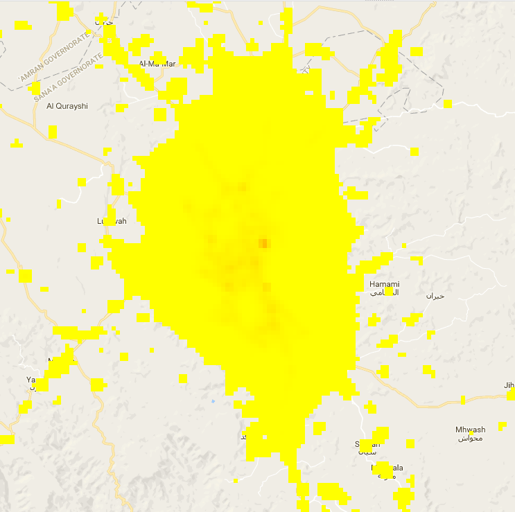
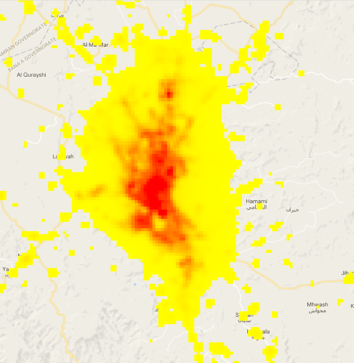
Having a look at the data
library(data.table)
library(foreign)
library(plyr)
library(parallel)

options(stringsAsFactors = FALSE)
setwd("/Users/thiemo/Dropbox/Research/Yemen")

# A DATA SET OF 34k populated places (or historically populated places)
YE <- data.table(read.csv(file = "~/Dropbox/Research/Yemen/Yemen-Cities.csv"))

# LIGHTS DATA IS FROM VIIRS Images made availabe on the Google Earth Engine
LIGHTS <- data.table(read.csv(file = "~/Dropbox/Research/Yemen/lightsall.csv"))

LIGHTS[, `:=`(year, as.numeric(substr(system.index, 1, 4)))]
LIGHTS[, `:=`(month, as.numeric(substr(system.index, 5, 6)))]
LIGHTS[, `:=`(.geo, NULL)]
LIGHTS[, `:=`(UFI, NULL)]
LIGHTS[, `:=`(LONGITUDE, NULL)]

LIGHTS[, `:=`(date, strptime(paste(year, month, "01", sep = "-"), "%Y-%m-%d"))]

LIGHTS <- join(LIGHTS, YE)
## Joining by: rownum
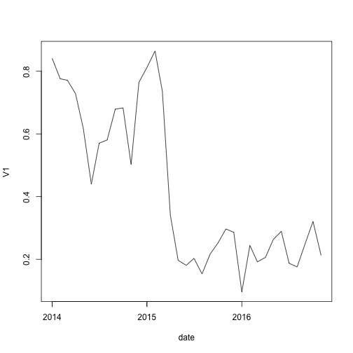
Some simple plots are quite suggestive. The following plots the average light emissions around populated places over time by month. The date of the intervention onset, which coincides with the date of the fall of Sana’a coincides with dramatic drop in light emissions.
Average lights dropped by a almost 2/3, suggesting a stand still in economic activity. Overall light emissions are still visible as indicated in the graphs suggesting that the places do not turn pitch black. The
plot(LIGHTS[, mean(list), by = date], type = "l")
The Distributional Effects of the Conflict
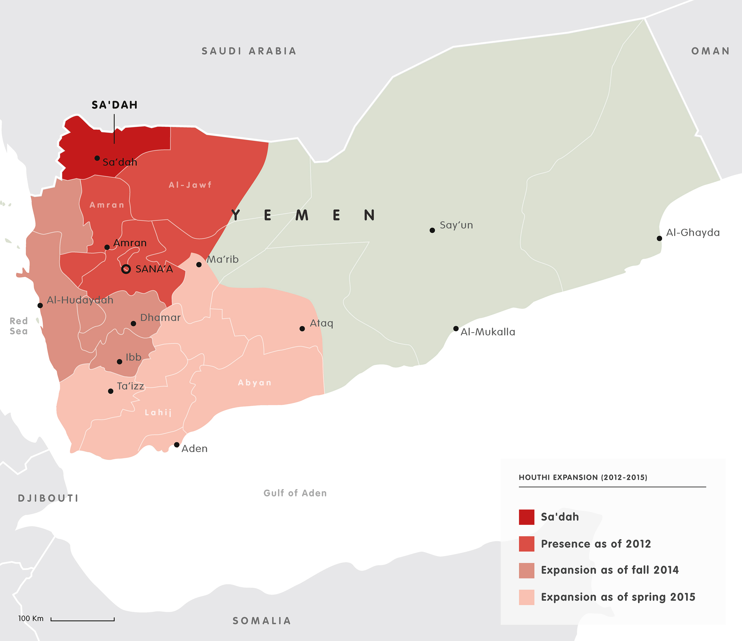
The Houthi movement has been gaining influence over a longer time period. In particular, since the 2012 the Houthi’s have gained influence spreading from North to the South. The European Council of Foreign Relations has produced maps illustrating the spatial expansion of Houthi control in Yemen.
A central question relates to the strategy of the Saudi military intervention. In particular, whether the intervention is aimed at territories that came under Houthi control since 2012 or whether the intervention is targeted at the Houthi-heartland.
A simple exercise that allows this study is to look at the evolution of lights in the northern Houthi-heartland relative to the populated places in the rest of the country that came under Houthi control since 2012.
A definition of what consists of the Houthi-heartland is subject to contention. But a conservative definition may consist of the four governerates Ammran, Sada’ah, Al Jawf and Hajjah.
LIGHTS[, `:=`(HOUTHI, as.numeric(ADM1 %in% c("15", "22", "21", "19")))]
require(ggplot2)
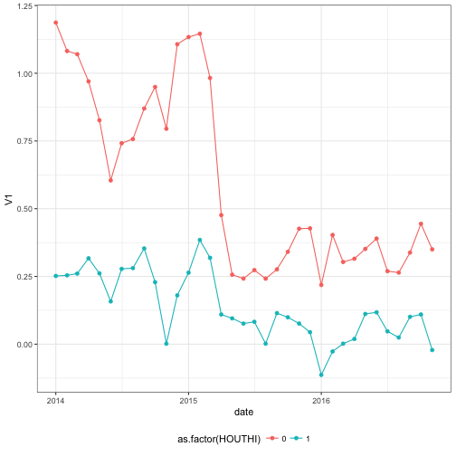
ggplot(LIGHTS[, mean(list), by = c("HOUTHI", "date")], aes(date, V1, colour = as.factor(HOUTHI))) +
    geom_line() + geom_point() + theme_bw() + theme(legend.position = "bottom")
The summary statistics suggest that in absolute terms much larger in the non-Houthi heartland. Though given that the initial level in the Houthi heartland is much lower, suggesting that that part of the country is much less developed. Given that there is a notional minimum light emissions of zero, this truncation of the data is a concern.
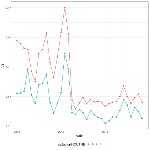
One way around this is to dummify the lights measure and look at whether a populated place is lit above a certain threshold.
LIGHTS[, `:=`(anylit, list > 0.25)]
ggplot(LIGHTS[, mean(anylit), by = c("HOUTHI", "date")], aes(date, V1, colour = as.factor(HOUTHI))) +
    geom_line() + geom_point() + theme_bw() + theme(legend.position = "bottom")
Again it is hard to see whether there is any divergence in trends in this dummified measure, but this naturally is less prone to be affected by the truncation inherent to this type of data.
A regression with location and time fixed effects that measures whether there was a distinct change in nightlights in places in the Houthi-heartland relative to the non-Houthi heartland suggests that there is indeed a marked difference, indicating that the conflict is concentrated in the non-Houthi heartland.
Definint the discrete variable for a difference in difference estimation and loading the lfe package that allows for high dimensional fixed effects:
LIGHTS[, `:=`(anylit, list > 0.25)]
LIGHTS[, `:=`(postKSAintervention, as.numeric(date > "2015-03-01"))]
library(lfe)
LIGHTS[, `:=`(date, as.factor(date))]
Running the actual difference in difference regressions:
# levels
summary(felm(list ~ postKSAintervention:HOUTHI | rownum + date | 0 | ADM1, data = LIGHTS))
##
## Call:
##    felm(formula = list ~ postKSAintervention:HOUTHI | rownum + date |      0 | ADM1, data = LIGHTS)
##
## Residuals:
##     Min      1Q  Median      3Q     Max
## -74.347  -0.205   0.043   0.194  82.063
##
## Coefficients:
##                            Estimate Cluster s.e. t value Pr(>|t|)
## postKSAintervention:HOUTHI   0.4184       0.1900   2.202   0.0277 *
## ---
## Signif. codes:  0 '***' 0.001 '**' 0.01 '*' 0.05 '.' 0.1 ' ' 1
##
## Residual standard error: 1.758 on 1172455 degrees of freedom
## Multiple R-squared(full model): 0.752   Adjusted R-squared: 0.7447
## Multiple R-squared(proj model): 0.003315   Adjusted R-squared: -0.02603
## F-statistic(full model, *iid*):  103 on 34519 and 1172455 DF, p-value: < 2.2e-16
## F-statistic(proj model): 4.848 on 1 and 22 DF, p-value: 0.03846
# dummified measure
summary(felm(anylit ~ postKSAintervention:HOUTHI | rownum + date | 0 | ADM1,
    data = LIGHTS))
##
## Call:
##    felm(formula = anylit ~ postKSAintervention:HOUTHI | rownum +      date | 0 | ADM1, data = LIGHTS)
##
## Residuals:
##      Min       1Q   Median       3Q      Max
## -1.12247 -0.10416  0.00593  0.06185  1.06958
##
## Coefficients:
##                            Estimate Cluster s.e. t value Pr(>|t|)
## postKSAintervention:HOUTHI  0.08470      0.02359    3.59  0.00033 ***
## ---
## Signif. codes:  0 '***' 0.001 '**' 0.01 '*' 0.05 '.' 0.1 ' ' 1
##
## Residual standard error: 0.2223 on 1172455 degrees of freedom
## Multiple R-squared(full model): 0.5762   Adjusted R-squared: 0.5637
## Multiple R-squared(proj model): 0.008458   Adjusted R-squared: -0.02073
## F-statistic(full model, *iid*):46.18 on 34519 and 1172455 DF, p-value: < 2.2e-16
## F-statistic(proj model): 12.89 on 1 and 22 DF, p-value: 0.00163
# taking logs
summary(felm(log(list) ~ postKSAintervention:HOUTHI | rownum + date | 0 | ADM1,
    data = LIGHTS[!is.infinite(log(list))]))
##
## Call:
##    felm(formula = log(list) ~ postKSAintervention:HOUTHI | rownum +      date | 0 | ADM1, data = LIGHTS[!is.infinite(log(list))])
##
## Residuals:
##      Min       1Q   Median       3Q      Max
## -12.8918  -0.3725   0.1060   0.5223   6.5958
##
## Coefficients:
##                            Estimate Cluster s.e. t value Pr(>|t|)
## postKSAintervention:HOUTHI   0.4133       0.1234    3.35 0.000809 ***
## ---
## Signif. codes:  0 '***' 0.001 '**' 0.01 '*' 0.05 '.' 0.1 ' ' 1
##
## Residual standard error: 0.8958 on 844476 degrees of freedom
##   (327294 observations deleted due to missingness)
## Multiple R-squared(full model): 0.6534   Adjusted R-squared: 0.6393
## Multiple R-squared(proj model): 0.01248   Adjusted R-squared: -0.02789
## F-statistic(full model, *iid*):46.12 on 34519 and 844476 DF, p-value: < 2.2e-16
## F-statistic(proj model): 11.22 on 1 and 22 DF, p-value: 0.002899
An alternative way to study this is by doing a flexible non-parametric estimation to rule out diverging trends prior to the military intervention.
summary(felm(anylit ~ date:HOUTHI | rownum + date | 0 | ADM1, data = LIGHTS))
##
## Call:
##    felm(formula = anylit ~ date:HOUTHI | rownum + date | 0 | ADM1,      data = LIGHTS)
##
## Residuals:
##      Min       1Q   Median       3Q      Max
## -1.12574 -0.10765  0.00313  0.06437  1.06515
##
## Coefficients:
##                       Estimate Cluster s.e. t value Pr(>|t|)
## date2014-01-01:HOUTHI       NA      0.00000      NA       NA
## date2014-02-01:HOUTHI  0.01095      0.01320   0.830 0.406641
## date2014-03-01:HOUTHI  0.03173      0.02764   1.148 0.250884
## date2014-04-01:HOUTHI  0.11048      0.06028   1.833 0.066814 .
## date2014-05-01:HOUTHI  0.09762      0.05271   1.852 0.063989 .
## date2014-06-01:HOUTHI  0.10249      0.05861   1.749 0.080336 .
## date2014-07-01:HOUTHI  0.07204      0.06053   1.190 0.233987
## date2014-08-01:HOUTHI  0.06338      0.04866   1.302 0.192778
## date2014-09-01:HOUTHI  0.03816      0.04690   0.814 0.415860
## date2014-10-01:HOUTHI  0.04247      0.04359   0.974 0.329930
## date2014-11-01:HOUTHI  0.05621      0.03646   1.542 0.123115
## date2014-12-01:HOUTHI  0.02213      0.03037   0.729 0.466205
## date2015-01-01:HOUTHI -0.02596      0.02585  -1.004 0.315415
## date2015-02-01:HOUTHI  0.02250      0.05141   0.438 0.661649
## date2015-03-01:HOUTHI  0.06080      0.05740   1.059 0.289437
## date2015-04-01:HOUTHI  0.13514      0.04806   2.812 0.004925 **
## date2015-05-01:HOUTHI  0.15874      0.04647   3.416 0.000635 ***
## date2015-06-01:HOUTHI  0.15493      0.05151   3.008 0.002632 **
## date2015-07-01:HOUTHI  0.12681      0.04697   2.700 0.006944 **
## date2015-08-01:HOUTHI  0.12363      0.04319   2.863 0.004202 **
## date2015-09-01:HOUTHI  0.13972      0.05276   2.648 0.008088 **
## date2015-10-01:HOUTHI  0.13422      0.04697   2.857 0.004273 **
## date2015-11-01:HOUTHI  0.12408      0.04566   2.717 0.006578 **
## date2015-12-01:HOUTHI  0.12125      0.04505   2.691 0.007119 **
## date2016-01-01:HOUTHI  0.11971      0.03905   3.065 0.002176 **
## date2016-02-01:HOUTHI  0.11952      0.04151   2.879 0.003984 **
## date2016-03-01:HOUTHI  0.12721      0.04239   3.001 0.002693 **
## date2016-04-01:HOUTHI  0.12537      0.04532   2.766 0.005669 **
## date2016-05-01:HOUTHI  0.12989      0.05297   2.452 0.014209 *
## date2016-06-01:HOUTHI  0.13070      0.05936   2.202 0.027675 *
## date2016-07-01:HOUTHI  0.14831      0.06597   2.248 0.024573 *
## date2016-08-01:HOUTHI  0.13047      0.04614   2.827 0.004693 **
## date2016-09-01:HOUTHI  0.14481      0.06024   2.404 0.016227 *
## date2016-10-01:HOUTHI  0.11782      0.05255   2.242 0.024959 *
## date2016-11-01:HOUTHI  0.12175      0.04473   2.722 0.006486 **
## ---
## Signif. codes:  0 '***' 0.001 '**' 0.01 '*' 0.05 '.' 0.1 ' ' 1
##
## Residual standard error: 0.2219 on 1172422 degrees of freedom
## Multiple R-squared(full model): 0.5776   Adjusted R-squared: 0.5652
## Multiple R-squared(proj model): 0.01175   Adjusted R-squared: -0.01738
## F-statistic(full model, *iid*): 46.4 on 34552 and 1172422 DF, p-value: < 2.2e-16
## F-statistic(proj model): 147.2 on 35 and 22 DF, p-value: < 2.2e-16
This suggests that the differential drop in lights occured only after March 2015, the month in which Saudi Arabia’s military intervention commenced.
On average, the regressions suggest that the drop in lights was significantly more pronounced outside the Houthi heartland. This suggests that the conflict and the bombing carried out by Saudi Arabia is mostly concentrated outside the Houthi rebel heartland.
That the dramatic drops in light emissions is associated with the Saudi military intervention is quite clear. The conflict between the Houthi rebels and the government had been ongoing for several years but only starting with the intervention of Saudi Arabia do marked differences between Houthi and non-Houthi heartland provinces appear.
This analysis can further be refined by studying the role of the religious make up of different provinces, as the role of the religious make up between Shia and Sunni muslim groups is said to be an important factor driving this conflict.
Nevertheless, this analysis suggests that high frequency satellite images such as these can be useful in assessing the extent to which areas area directly affected by conflict, which may be useful for targeting humanitarian relief.
